2025 Science Journal

Senior Editor

Dr Matthew Hill

Creative Direction

Mrs Susan Layton

Dr Matthew Hill

Research Supervisors

Mrs Kathy Haigh

Dr Matthew Hill

The Barker Institute

About the Scientific Research in School Journal

When the New South Wales Education Standards Authority announced a new course “Science Extension” to commence in 2019 we were thrilled that there was an opportunity for a formally asessed capstone experience in Science for our students. From the perspective of the Barker Institute it was an exciting chance to support students doing academic research, alongside other subjects such as History Extension, Music Extension and English Extension 2.

Where many capstone project courses fail is the at final step of the research process – dissemination. Research is not merely the process of conducing an investigation and writing a report, but sharing it with the wider community so that people can learn, critique, have other student researchers at multiple schools build on the projects published. I am so glad to be able to publish this journal each year now celebrating 111 articles, each representing genuine contributions to science.

Dr Matthew Hill Director, Barker Institute Senior Editor, Scientific Research in School

Introduction

The essence of scientific inquiry lies not merely in the accumulation of facts, but in the cultivation of minds capable of questioning, hypothesizing, and discovering. Barker’s Science research program continues to embody this principle, empowering students to engage in authentic scientific investigation that contributes meaningfully to our collective understanding of the natural world.

The quality of a school like Barker is measured inter alia by the intellectual achievements of its students and by their capacity to address the challenges facing our world. In 2025, our student researchers have once again demonstrated exceptional scientific acumen, conducting investigations that exemplify the rigorous methodology, analytical thinking, and innovative problem-solving that define genuine scientific research.

Under the expert mentorship of our research professionals, this cohort of young scientists has engaged with complex scientific questions, employed sophisticated research methodologies, and generated findings that advance our understanding of phenomena ranging from the molecular to the cosmic scale. Their work demonstrates not only technical competence but also the intellectual curiosity and persistence essential to scientific discovery.

This seventh volume of Scientific Research in School represents more than academic achievement – it showcases the development of the next generation of scientific minds. These students have learned to formulate testable hypotheses, design-controlled experiments, analyse data with statistical rigor, and communicate their findings with clarity and precision.

The research presented in these pages reflects the diversity and depth of contemporary scientific inquiry. From investigations into environmental sustainability to explorations of emerging technologies, our students have tackled questions with real-world implications. Their work demonstrates that meaningful scientific research is not confined to university laboratories or corporate research centres – it can emerge wherever curious minds are given the tools and freedom to explore.

As we face an era of unprecedented global challenges – from climate change to biodiversity loss, from emerging diseases to technological disruption – the importance of fostering scientific literacy and research capability in young people cannot be overstated. The students whose work appears in this volume represent hope for our collective future, equipped not only with knowledge but with the scientific mindset necessary to address the complex problems that await them.

I am immensely proud of these young researchers and their commitment to excellence in scientific investigation. Their achievements remind us that when we provide students with authentic opportunities to engage in scientific research, we invest not only in their individual development but in the future of scientific discovery itself.

“Science is not only a disciple of reason but, also, one of romance and passion. The future depends on our ability to understand our world through the inquiry and reasoning that science provides.” –Stephen Hawking

The work presented in this journal embodies that passion and reasoning, offering hope that the future of both scientific knowledge and planetary stewardship rests in capable hands.

Mr Phillip Heath AM Head of Barker College

Science at Barker is a shared journey of curiosity and growth, culminating in student-led research that reflects the strength of our student body and the dedication of our educators.

Science is for everyone. Across our community – for primary school students, secondary school students, teachers, and parents – we are pleased to provide opportunities for thinking scientifically and engaging with the world through experimentation and inquiry. This Journal represents the capstone, but the journey is a long-term process. Every day, in hundreds of science classes at Barker, students experience continuous growth, supported by a superb team of teachers. I regularly witness students of all ages investigating complex topics by designing fair tests, collecting data, and reasoning their conclusions.

It is a privilege to pursue Science within such a vibrant and supportive community, and to share our research publicly. We invite you to read, reflect, offer feedback, and even build upon these projects in your own contexts.

Research Supervisors

I am grateful for the work of all Science staff at Barker for their investment in the Science Extension students. In particularly I want to honour and thank the two research supervisors, Dr Matthew Hill and Mrs Kathy Haigh, who along with outstanding laboratory staff, supported these students through the Science Extension research program.

Mrs

Virginia Ellis

Head of Science

In these 14 academic articles, students wrestle with the extant literature to accurately describe a gap in scientific understanding, before implementing valid methods to produce novel, first-hand results and findings to address this gap. It has been a pleasure to journey with them and wrestle with complex ideas and communication. Together we have endured through complications, celebrated breakthroughs, and explored implications.

We are incredibly proud of them personally, and also the work that they have produced. We look forward to seeing the impact of this work on future research in Science.

PART 1: CHEMISTRY

Synthesis of 4-(4-chloropyridin-2-yl)-N-(5-chloropyridin-2-yl)thiazol-2-amine for the Treatment of Mycetoma

Josiah Chan

The Effect Ultraviolet Light Exposure has on the Anthocyanin content within Purple Heart plants (tradescantia pallida)

Huxley Hall

Effects of Pre-Harvest UV-C Hormesis on Lycopene Production in Tomato Plants

Kevin Sun

PART 2: PHYSICS AND DATA SCIENCE

The Effects of Ultraviolet Light Exposure on the Ultimate Tensile Strength of Common 3D Printing Polymers

Jack Moon FFF ABS Layer height interaction with thermal annealing effects

Nicholas

Angus

into the Efficiency of Novel Toroidal Propellers in Ground Effect

The Aerodynamic Performance of Two Hot Stages for Starship Super Heavy

Effect of a Stern Mounted Drag Reduction Superstructure on Post-Panamax Maritime Cargo Vessels

Josh McLean

Affluence and Mobility: Investigating traffic volume changes in Sydney during the 2020 and 2021 COVID-19 Lockdowns

Roy Yan

PART 3: BIOLOGY AND EARTH & ENVIRONMENTAL SCIENCE

Does Glyphosate application affect pollinator visitation on Round-Up ready Tru-Flex Canola

Eddy Phillips

Geographic Variation in Eastern Brown Snakes (Pseudonaja Textilis) venom composition: An analysis of current research 105

Bowen Doak

What role does ecological adaptation play in the development of tool-use behaviour in Choerodon wrasses? 117

Ally Habgood

Biofiltration of agricultural runoff using Carrex Apressa 123

Brett Minkus

How do different postharvest treatments (sugar, bleach, water regulation) effect the vase life and colour stability of white carnations, measured by CIELAB colorimetry?

Melissa Li

129

Chemistry

This year, students undertook three diverse and impactful projects, applying their knowledge of chemistry and biochemistry.

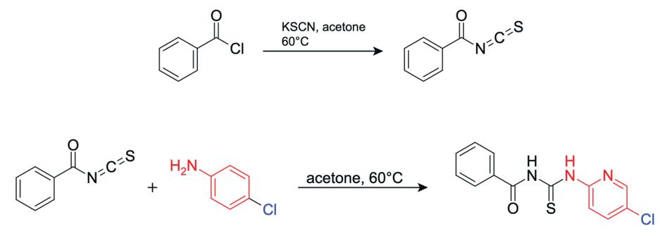
Barker College continued its active participation in the Breaking Good citizen science project, a collaboration with the Open Source Mycetoma Consortium focusing on discovering new treatments for mycetoma, a neglected tropical disease. Josiah’s project aimed to synthesise a novel 2-aminothiazole analogue. By incorporating chlorine substituents on both pyridine rings, he successfully created a high-purity compound with a satisfactory yield. This new molecule is now ready for efficacy testing, an important step toward finding a new treatment for this debilitating disease.

Building on the understanding that antioxidants combat disease, two student projects investigated the effect of ultraviolet (UV) light exposure on the antioxidant content of plants. Huxley’s project found a relationship between UV exposure and anthocyanin content in the Purple Heart plant (Tradescantia pallida), whilst Kevin’s project also showed an effect of UV-C on lycopene production in tomatoes, with both projects identifying an optimal exposure time for maximising antioxidant levels.

Synthesis of 4-(4-chloropyridin-2-yl)-N-(5-chloropyridin-

2-yl)thiazol-2-amine for the Treatment of Mycetoma

Josiah Chan

Barker College

Mycetoma is a granulomatous disease that spreads to skin, deep tissues and bone. It has been recorded as a neglected tropical disease, with a lack of short term medication for eumycetoma, typically requiring antifungal treatment followed by surgical intervention. The scientific report outlines the synthesis of an analogue of 2-aminothiazole with substitution of chlorine on both pyridine rings to be tested in vitro against M. mycetomatis. The compound was successfully synthesised, with a 43% overall yield, and a high purity as determined by 13C-NMR and 1H-NMR. Due to time constraints, the in vitro results of the product are pending and will be required to determine its antifungal efficacy.

Literature Review

Mycetoma is a chronic, granulomatous disease of the subcutaneous tissue and skin that spreads to affect the skin, deep tissues, and bone (WHO, 2022). It is characterised by a symptomatic triad of tumour, fistulas and the formations of grains. It typically affects the lower extremities, but it can occur in almost any region of the body (Vera-Cabrera, 2021). Mycetoma was officially to be a neglected tropical disease (NTD) by the World Health Organisation in 2016, prevalent in the tropical and subtropical regions, popularly known as the “Mycetoma Belt” (30N to 15 S latitude) (Agarwal et al., 2021). The endemic areas are characterised by short rainy reasons with little daily temperature fluctuations, followed by long dry seasons with broad daily temperature fluctuations of 45-60 °C to 15-18 °C (Reis & Reis-Filho, 2018). The extreme alteration in weather conditions suggests that it may be a prerequisite to the survival of the causative organism in its natural niche (Ahmed et al., 2004). As such, in a comprehensive literature review by Emery & Denning (2020), tropical countries Sudan, Mexico, and India are reported to have the highest number of cases with 10608, 4155 and 1116 individuals reported respectively. Mycetoma has been contracted by individuals in 102 countries, many outside the “Mycetoma Belt”, (Figure 1) but many countries only reported a single case. The disease has reported a total of 19494 cases from 1876 to 2019 (Emery & Denning, 2020)

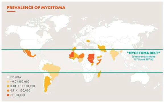
1: Prevalence of mycetoma (Source: DNDi 2019 adapted from van de Sande WWJ).

Mycetoma can be caused by specific groups of fungi or by bacteria; therefore, it is classified into eumycetoma and actinomycetoma respectively. Eumycetoma is commonly found in areas with lower rainfall and less variation in temperature, whilst actinomycetoma is more commonly observed in areas with higher rainfall and lower temperatures (Chandler et al., 2023a). Actinomycetoma is commonly treated with a combination of antibiotics, including dapsone (Figure 2) and TMP-SMX daily for 2 to 3 years. Other effective treatments include aminoglycosides (such as amikacin and streptomycin) as well as quinolones (Arenas et al., 2017)

On the other hand, eumycetoma poses more significant public health challenges due to the lack of

effective short-term medication available. Literature identifies the fungus Madurella mycetomatis (M. mycetomatis) as the leading causative agent for Eumycetoma. However, over 50 species of mycetoma-causative fungi have been reported around the world, with patients simultaneously infected with multiple fungi (Hashizume et al., 2022). Currently, treatment for eumycetoma is preoperative antifungal treatment for six months followed by surgical intervention, usually in the form of adequate wide local excision, repeated aggressive debulking or amputation in advanced disease. 400 mg/day itraconazole is recommended as the first line drug with lesions of moderate and large sizes and supported by surgical excision. However, despite prolonged treatment with itraconazole before and after surgery, postoperative recurrence is quite common, with at least 33% recurrence rate among patients (Siddig et al., 2021). Further, even though M. mycetomatis is highly susceptible to itraconazole in vitro, grains containing fungi were isolated from patients on prolonged treatment with itraconazole, highlighting that itraconazole may only limit the extent of the infection instead of complete eradication of the M. mycetomatis tissue burden (Siddig et al., 2021) Eumycetoma patients often present to treatment at late stages of the advanced disease, which is attributed to the substantial lack of health education and health facilities in low-socioeconomic areas where eumycetoma is endemic (Elkheir et al., 2020)

In vitro susceptibility assays were developed for many of the causative agents of the black grain eumycetoma, showing a low 50% minimum inhibitory concentration (MIC50) for the azoles and higher MICs for amphotericin B (MIC50 0.5μg/mL) (Chandler et al., 2023b) In vivo activity was also tested in a larva model developed by Wendy W J van de Sande, in where the larvae of Galleria mellonella are inoculated by injected a suspension of viable M.mycetomatis into the last left pro-leg (Lim et al., 2018). This in vivo testing further confirmed the inefficiency of treatments such as itraconazole and ketoconazole. Thus, an effective and affordable treatment for eumycetoma is yet to be found.

The Mycetoma Open Source Project (MycetOS) uses an ‘open source pharma’ approach to discover new treatments target M.mycetomatis. The 2aminothiazoles are a group of compounds that have been identified as potential family of molecules which could be effective at treating eumycetoma (Figure 3), first identified by the screening of the stasis box, a box of 400 drug like compounds provided free of charge by the Medicines for Malaria Venture (MMV) (Lim et al., 2018)

3: Graphical abstract of applications to 2aminothiazole derivatives (Source: Das et al., 2016)

Generally, 2-aminothiazole derivatives are known for their broad antimicrobial effects (Figure 3). Their core structure is found compounds active against bacteria, fungi and even prions. Researchers at the Open Source Mycetoma Project have found that having chloro substituent on the pyridine N gave the lowest IC50 as well as a chlorine substituent on the left-hand (bromoketone derived) side gave the best results. Furthermore, the presence of chlorinated pyridine rings have shown significant activity against E. Coli and Candida albicans. A recent study showed compounds containing chlorinated pyridine rings (ie. Methyl (2-((5-chloropyridin-2-yl)amino)-2oxoacetyl)glycinate) demonstrated potent antibacterial activity against E. coli, with MIC values of 25μg/mL, whilst similar compounds exhibited the most potent antifungal activity against C. albicans with MIC values of 250 μg/mL. (Kanjariya et al., 2025). Furthermore, halogenated compounds – such as chlorine substituents – are known to increase lipophilicity as they facilitate passive diffusion across lipid membranes and enhance oral bioavailability (Fraley & Sherman, 2018;Silverman & Holladay, 2014). Thus, by working with the Breaking Good team, 4-(4-chloropyridin-2-yl)-N-(5-chloropyridin-2yl)thiazol-2-amine has been determined as a potential compound to be tested in vitro against M. Mycetomatis.

Figure 4: Structure of 4-(4-chloropyridin-2-yl)-N-(5chloropyridin-2-yl)thiazol-2-amine

The precise mechanism for which 4-(4-chloropyridin2-yl)-N-(5-chloropyridin-2-yl)thiazol-2-amine exert antifungal effects is currently undetermined, however literature shows the 2-aminothiazole compound as potent calcium-activated potassium (KCa) channel inhibitor in humans (Gentles et al., 2008). The proteins regulate calcium ions that bind to calmodulin, leading to the higher occupancy opening the KCa channel. This opening results in a hyperpolarisation of the plasma membrane and significantly affects the rate and pattern of neuronal firing, killing the pathogen. (Gentles et al., 2008). Further, novel 2-aminothiazoles have shown to be inhibitors of multiple enzyme targets such as EGFR/VGFER kinase, Akt (PKB) protein kinase, and others (Alizadeh & Hashemi, 2021). The chloropyridine in the structure can enhance binding through hydrophobic interactions or halogen bonding with the target enzyme’s active site, thereby increasing potency. Moreover, the Chloropyridine contributes to a higher Log D (lipophilicity) which has been correlated with better penetration of the thick mycetoma grain material and fungal biofilms (Van de Sande, 2022)

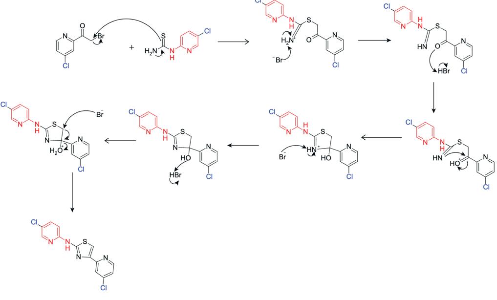
The synthesis of 4-(4-chloropyridin-2-yl)-N-(5chloropyridin-2-yl)thiazol-2-amine undergoes the Hantzsch thiazole condensation reaction, commonly used by other researchers in the Open Source Mycetoma Project. It is an organic reaction that synthesises thiazole derivatives, particularly 2aminothiazoles by condensing a haloalkane (specifically, a bromoketone) with a thiourea or thioamide.

The general reaction scheme is as follows:

α-Haloketone + Thiourea  2-Aminothiazole Derivative

Scientific Research Question

Can a chloropyridine analogue of 4-(4-chloropyridin2-yl)-N-(5-chloropyridin-2-yl)thiazol-2-amine be synthesised with a high yield to be tested in vitro against M. mycetomamatis?

Scientific Hypothesis

The higher the moisture content of all three composites (of the 3D print

A chloropyridine analogue of 4-(4-chloropyridin-2yl)-N-(5-chloropyridin-2-yl)thiazol-2-amine can be successfully synthesised in a school lab with a

sufficient yield and purity to be tested as an anti-fungal agent in vitro against M. mycetomatis.

Methodology

1. Synthesis of (N-((5-chloropyridin-2yl)carbamothioyl)benzamide

Figure 5: Structural formula of N-((5-chloropyridin-2yl)carbamothioyl)benzamide

Potassium thiocyanate (4.54g, 47.67n mmol, 1.2 equiv) was added to a round bottom flask with a reflux condenser, washed in acetone (90mL). Benzoyl chloride (6.15g, 43.556mmol, 1.12 equiv) was added to the reflux condenser and the reaction was heated to reflux (60°C) and stirred for one hour. 5-choropyridin-2-amine (5.00g, 38.89mmol, 1 equiv) was added and the reaction was returned to reflux for another two hours. The reaction was poured over 100mL of ice water and stirred for 10 minutes. TLC was conducted with 20% EtOAc/hexane as the eluent. The precipitation was collected by vacuum filtration, washed with ice water and dried in a dessicator overnight to afford N-((5-chloropyridin-2yl)carbamothioyl)benzamide (Figure 4) as a pale solid (11.37g, quantitative yield).

2. Hydrolysis to synthesise 1-(5-chloropyridin-2yl)thiourea

Figure 6: Structural formula for 1-(5-chloropyridin-2yl)thiourea

N-((5-chloropyridin-2-yl)carbamothioyl)benzamide (10.7g, 36.67mmol, 1 equiv) was added to a round bottom flask fixed with a reflux condenser with 2.5M aqueous NaOH solution (90mL, 225mmol, 6.13 equiv). The reaction was refluxed at 80°C for 2 hours with stirring. 1M HCl was added dropwise to adjust the pH to be within 4.0~5.0 to remove the remaining NaOH. Saturated Na2CO3 solution was added to adjust the pH to 8.0 to precipitate the product. The precipitate was then collected via vacuum filtration and washed

with cold water (25mL), then dried overnight in a desiccator to afford 1-(5-chloropyridin-2-yl)thiourea (Figure 5) as a white, flaky crystalline solid (3.95g, 57.39% yield).

3. Cyclisation to 4-(4-chloropyridin-2-yl)-N-(5chloropyridin-2-yl)thiazol-2-amine

7: 4-(4-chloropyridin-2-yl)-N-(5-chloropyridin-2yl)thiazol-2-amine.

1-(5-chloropyridin-2-yl)thiourea (3.84g, 20.46mmol 1 equiv) and 2-bromo-1-(4-chloropyridin-2-yl)ethan-1one (5.00g, 21.32mmol. 1.05 equiv) was added to a round bottom flask fitted with a condenser in 100mL of ethanol. The reaction was heated to reflux at 80°C and stirred until completion, determined by TLC (20% EtOAc/hexane). The mixture was cooled by adding 65mL ice water. Saturated Na2CO3 solution was added to adjust the pH to 8.0 to precipitate the product. The precipitate was then collected via vacuum filtration and washed with cold water (2 x 10mL), then dried overnight in a desiccator to afford 4-(4chloropyridin-2-yl)-N-(5-chloropyridin-2-yl)thiazol2-amine. Analytical characterisation of 1H-NMR, 13CNMR, TLC, HPLC, and LRMS was conducted on both intermediate compounds and the final compound.

Results

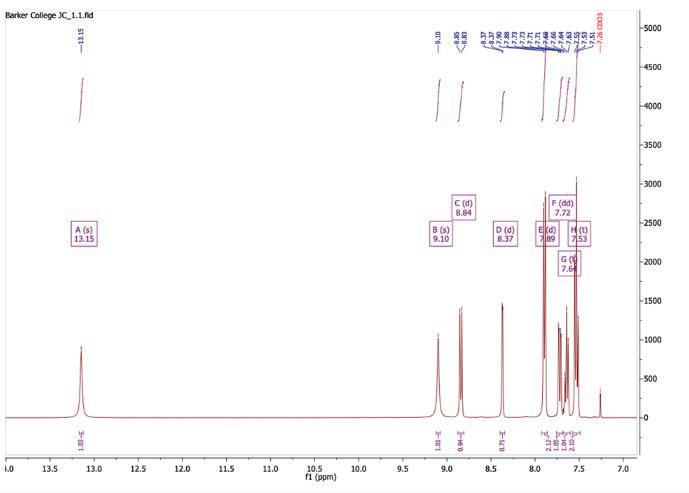
Figure 8: 1H NMR spectrum after step 1

1H NMR (400 MHz, Chloroform-d) δ 13.15 (s, 1H), 9.10 (s, 1H), 8.84 (d, J = 8.8 Hz, 1H), 8.37 (d, J = 2.6 Hz, 1H), 7.89 (d, J = 7.8 Hz, 2H), 7.72 (dd, J = 8.9, 2.6 Hz, 1H), 7.64 (t, J = 7.4 Hz, 1H), 7.53 (t, J = 7.6 Hz, 2H).

Table 1: 1H-NMR spectrum after step 1

Peak (ppm) Integral Splitting Assignment

13.15 1 Singlet

NH adjacent to benzoyl C=O (strongly deshielded due to conjugation and H-bonding)

9.10 1 Singlet NH adjacent to carbonyl group

8.84 1 Doublet H on pyridine ring, ortho to N and meta to Cl

8.37 1 Doublet H on pyridine ring, meta to N and ortho to Cl

7.89 2 Doublet H on benzene ring, ortho to CONH group

7.72 1 Doublet of doublets H on benzene ring, meta to CONH group

7.64 1 Triplet H on benzene ring, para to CONH group

7.53 2 Triplet H-3 and H-5 on phenyl ring

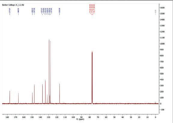
9: 13C NMR spectrum after step 1

13C NMR (101 MHz, CDCl3) δ 177.07, 166.51, 149.53, 147.26, 137.27, 133.85, 131.52, 129.24, 128.56, 127.60, 116.58.

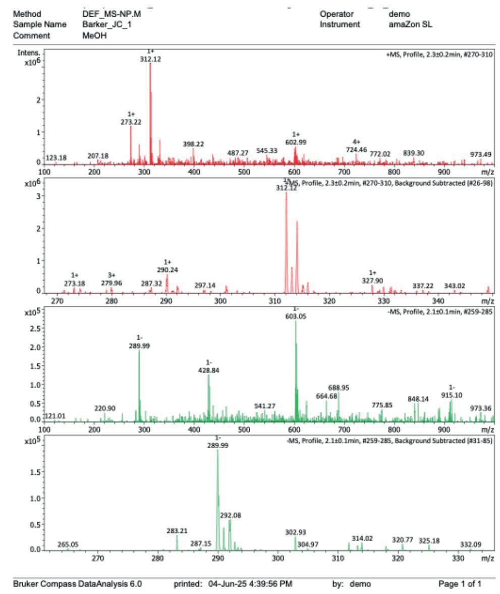
10: Mass spectrum after step 1

[ESI+] m/z 312.12 [M+Na]+, single chlorine isotope pattern present

[ESI-] m/z 289.09 and 292.08 [M-H]-, single chlorine isotope pattern present

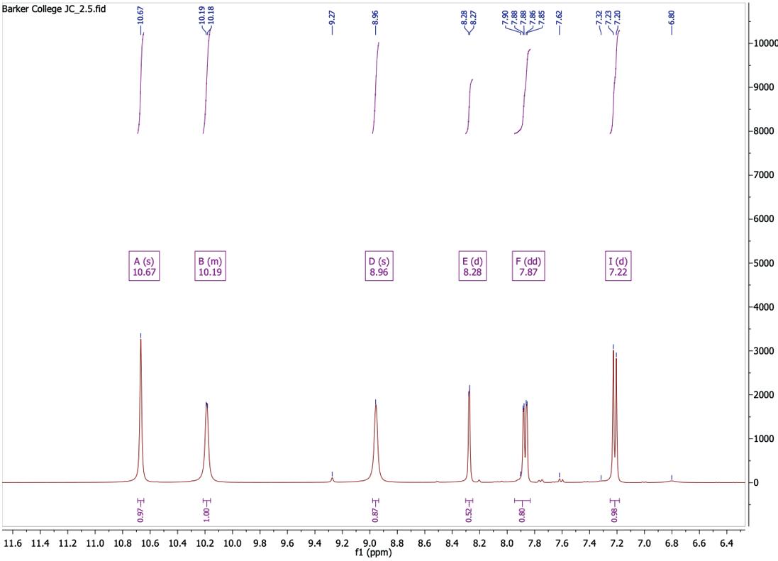
Figure 11: 1H NMR spectrum after step 2

1H NMR (400 MHz, DMSO-d6) δ 10.67 (s, 1H), 10.21 – 10.16 (m, 1H), 8.96 (s, 1H), 8.28 (d, J = 2.6 Hz, 1H), 7.87 (dd, J = 8.9, 2.7 Hz, 1H), 7.22 (d, J = 8.9 Hz, 1H).

Table 2: 1H-NMR spectrum after step 2

Peak (ppm) Integral Splitting

10.67 1 Singlet

10.19 1 Multiplet

8.96 1 Singlet

8.28 1 Doublet

7.87 1 Doublet of doublets (J = 8.9, 2.7 Hz)

7.22 1 Doublet (J = 8.9 Hz)

Assignment

NH proton adjacent to C=S

NH adjacent to pyridine ring

Aromatic proton ortho to NH on pyridine ring

Aromatic proton adjacent to Cl on pyridine

Pyridine protons between N and Cl

Aromatic proton para to NH on pyridine

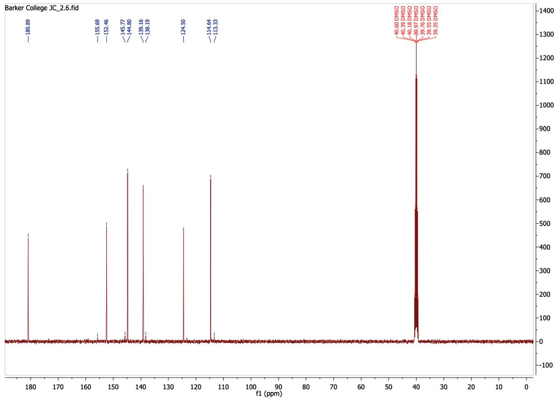
NMR (101 MHz, DMSO) δ 180.89, 152.46, 144.80, 139.16, 124.50, 114.64.

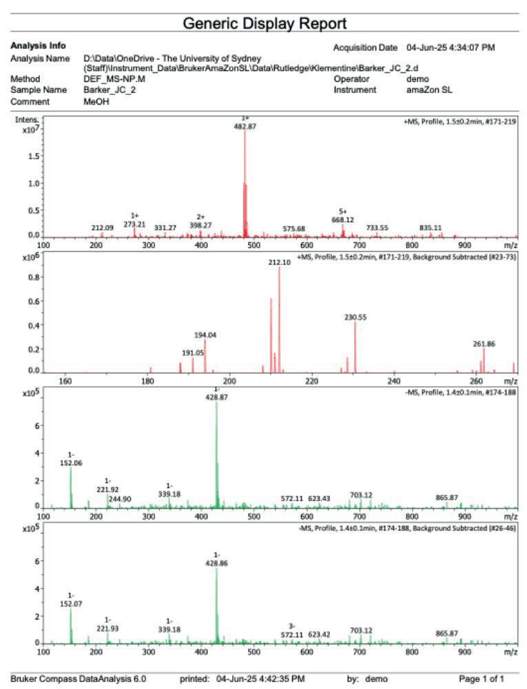
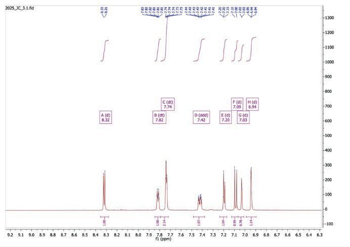
Figure 14: 15: 1H NMR spectrum after step 3

1H NMR (500 MHz, Toluene-d8) δ 8.32 (d, J = 6.4 Hz, 1H), 7.82 (dt, J = 6.3, 2.0 Hz, 1H), 7.74 (dt, J = 4.2, 1.7 Hz, 1H), 7.42 (ddd, J = 9.4, 3.8, 2.2 Hz, 1H), 7.20 (d, J = 5.6 Hz, 1H), 7.09 (d, J = 9.4 Hz, 1H), 7.03 (d, J = 1.7 Hz, 1H), 6.94 (d, J = 1.7 Hz, 1H

Table 3: 1H-NMR spectrum after step 3

Peak (ppm) Integral Splitting Assignment

8.32 1 Doublet H at position 3of the right pyridine ring

7.82 1 Doublet of triplets H at position 3 of the left pyridine ring

7.74 2* Doublet of triplets Overlapping signals of H-4 of left pyridine and toluene solvent

7.42 1 Doublet of doublet of doublets H-5 of left pyridine ring showing multiple couplings

7.20 1 Doublet H-6 of right pyridine ring

7.09 1 Doublet H-5 of right pyridine ring

7.03 1 Doublet H-4 of right pyridine ring

6.94 1 Doublet NH proton between thiazole and right pyridine ring

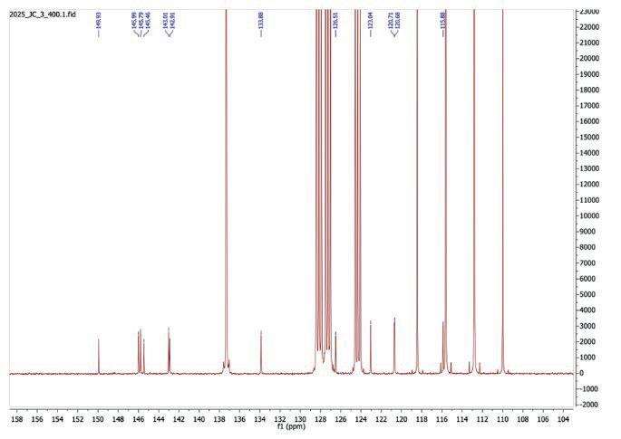
15: 13C NMR spectrum after step 3

13C NMR (101 MHz, Toluene-d8) δ 149.93, 145.99, 145.79, 145.46, 143.01, 142.91, 133.88, 126.51, 123.04, 120.71, 120.68, 115.88

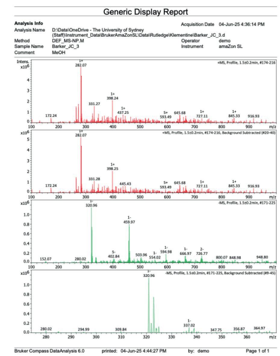
16: Mass spectrum after step 3

[ESI+] m/z no relevant adducts seen [ESI-] m/z 320.96 [M-H]-, double chlorine isotope pattern present

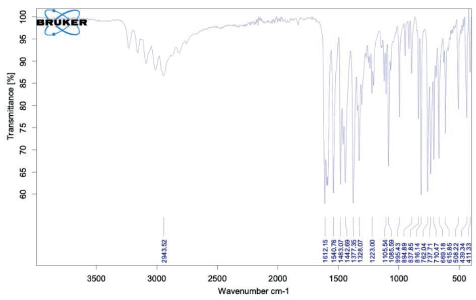
Figure 17: IR spectroscopy after step 3

Final Product characterisation results:

LRMS [ESI-]: m/z 320.96 [M-H]- FTIR (ATR) νmax/cm-1: 3234, 3158, 3090, 3009, 2946, 2815, 2756, 1612, 1541, 1483, 1443, 1377, 1328, 1223, 1106, 1086, 995, 895, 838, 816, 762, 738, 710, 669, 616, 508, 439, 411. 1H NMR (500 MHz, Toluene-d8) δ 8.32 (d, J = 6.4 Hz, 1H), 7.82 (dt, J = 6.3, 2.0 Hz, 1H), 7.74 (dt, J = 4.2, 1.7 Hz, 1H), 7.42 (ddd, J = 9.4, 3.8, 2.2 Hz, 1H), 7.20 (d, J = 5.6 Hz, 1H), 7.09 (d, J = 9.4 Hz, 1H), 7.03 (d, J = 1.7 Hz, 1H), 6.94 (d, J = 1.7 Hz, 1H). 13C NMR (101 MHz, Toluene-d8) δ 149.93, 145.99, 145.79, 145.46, 143.01, 142.91, 133.88, 126.51, 123.04, 120.71, 120.68, 115.88.

Table 4: Mass spectroscopy for compounds 1 and 3

Compound Actual mass Mass seen Adduct

JC_1 291.023 289.99- [M-H]-

JC_3 321.985 320.96- [M-H]-

Table 5: Yield and purity for compound 1, 2 and 3

Compound Yield Purity by HPLC (%) Appearance

JC_1 11.37g, 100% 97.31 Pale solid

JC_2 3.95g, 57.39% 99.41% Crystalline white solid

JC_3 5.41g, 81.92% Not conducted Light brown solid

Discussion

Step 1: Synthesis of (N-((5-chloropyridin-2yl)carbamothioyl)benzamide

18: Structural equations for the reaction of step 1

In step 1, potassium thiocyanate (KSCN) reacts with benzoyl chloride. The nitrogen atom attacks the carbonyl carbon of benzoyl chloride, pushing electrons onto the oxygen and forming a tetrahedral intermediate, which collapses as the carbonyl reforms and chlorine is expelled, producing benzoyl isothiocyanate (Figure 18).

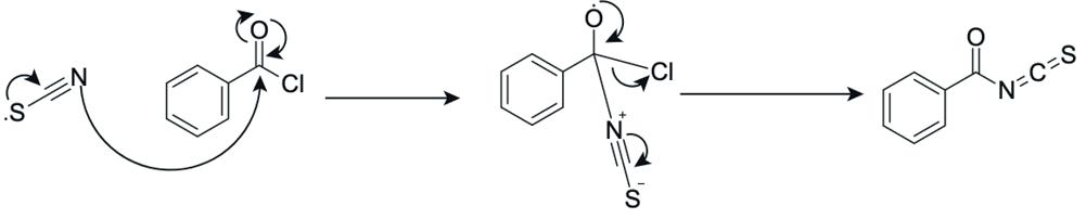
Figure 19: Reaction to form benzoyl isothiocyanate

The starting material, 5-chloropyridin-2-amine (in red) is then reacted with benzoyl isothiocyanate, whereby the nitrogen atom of the starting material attacks the electrophilic carbon of the isothiocyanate group. The C=N double bond of the isothiocyanate group shifts electrons to the nitrogen, forming a tetrahedral intermediate, and after electron rearrangement produces N-((5-chloropyridin-2yl)carbamothioyl)benzamide (Figure 19).

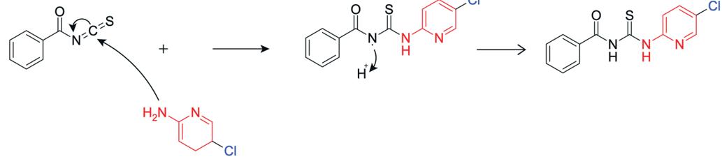
Figure 20: Reaction to form N-((5-chloropyridin-2yl)carbamothioyl)benzamide

N-((5-chloropyridin-2-yl)carbamothioyl)benzamide was produced successfully with a quantitative yield. The negative ion mass spectrometry (Figure 9) indicated the production of a compound with 289.99 [M-H]- molecular mass, which corresponds to the actual mass of the benzamide compound at 291.023. The 13C-NMR (Figure 8) displays 11 peaks, matching to the number of carbon environments in the final product. The 1H-NMR spectrum (Figure 7) of N-((5chloropyridin-2-yl)carbamothioyl)benzamide shows a singlet at 9.10 ppm corresponding to the amide NH proton adjacent to the carbonyl group. Doublets at 8.84 and 8.37 ppm are assigned to aromatic protons on

the 5-chloro-pyridin-2-yl ring, deshielded by the adjacent nitrogen and chlorine atoms. Peaks between 7.89 and 7.53 ppm correspond to the five aromatic protons on the benzoyl ring. The HPLC (Figure 23) indicated that the reaction was successful with a 97.31% purity. In combination of all results, it can be concluded that N-((5-chloropyridin-2yl)carbamothioyl)benzamide was successfully synthesised.

Step 2: Hydrolysis to synthesise 1-(5chloropyridin-2-yl)thiourea

In step 2, a hydrolysis reaction occurs where the lone pair on the hydroxide ion attacks the electrophilic carbon on the benzoyl carbonyl group, forming a tetrahedral intermediate. The lone pair on the negatively charged oxygen reforms the carbonyl, pushing electrons onto the amide nitrogen, causing cleavage of the C-N bond between the carbonyl carbon and the NH group, breaking the benzamide linkage. The cleaved fragment is stabilised via protonation of the leaving NH group, yielding 1-(5chloropyridin-2-yl)thiourea (Figure 21).

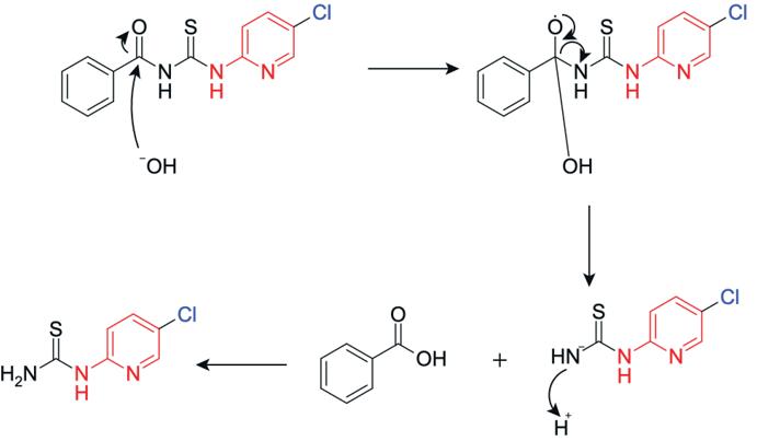
Figure 22: Reaction to form 1-(5-chloropyridin-2yl)thiourea

1-(5-chloropyridin-2-yl)thiourea was produced successfully with a yield of 57.39%, which is consistent with the yield obtained by compounds synthesised using Hantzsch condensation reaction. The low yield is most likely due to the reaction not going to completion, where the reaction priorities the purity of the compound rather than yield. The 13CNMR (Figure 11) displays 6 peaks, matching to the number of carbon environments in the final product. The carbon peaks at lower ppm are due to the organic solvent DMSO. The 1H-NMR spectrum (Figure 10) displays distinct downfield peaks, with the singlet at

10.67 ppm was assigned to the NH proton adjacent to the C=S group, while the broad multiplet at 10.19 ppm corresponds to the NH proton connecting the pyridine ring to the thiourea moiety, both signals being highlight deshielded due to adjacent electronegative atoms. The singlet at 8.96 ppm is assigned to the C-3 hydrogen on the pyridine ring, and the remaining peaks at 8.28ppm (d), 7.87 (dd), and 7.22 (d) are attributed to the other aromatic protons (C-4, C-5, and C-6) of the pyridine ring. The HPLC (Figure 24) indicated the compound had a purity of 99.41%, consistent with results obtained by similar experiments. The mass spectroscopy conducted (Figure 12) showed unknown adduct at 428.86 [ESI-] and the molecular mass was unable to be identified, however due to the other analysis the compound was likely synthesised. Thus, from the results, 1-(5chloropyridin-2-yl)thiourea was successfully synthesised with a high purity.

Step 3: Cyclisation to 4-(4-chloropyridin-2-yl)-N(5-chloropyridin-2-yl)thiazol-2-amine

2-bromo-1-(4-chloropyridin-2-yl)ethan-1-one was reacted with 1-(5-chloropyridin-2-yl)thiourea to produce 4-(4-chloropyridin-2-yl)-N-(5-chloropyridin2-yl)thiazol-2-amine as the final compound. The thiourea sulfur attacks the carbonyl carbon, displacing the bromide ion and forms a tetrahedral intermediate. The proton shift stabilises the intermediate and the lone pair on the adjacent nitrogen picks up a proton. The system stabilises through a proton transfer and

expulsion of HBr. The intermediate undergoes further proton transfers and elimination of water, finalising the aromatic thiazole structure, producing 4-(4chloropyridin-2-yl)-N-(5-chloropyridin-2-yl)thiazol2-amine.

The negative ion mass spectrometry (Figure 15) indicated the production of a product of molecular mass 321.985[M-H]-, which is in within similar size of the expected 320.96 molecular weight. The double chlorine isotope pattern was present at m/z 320.96 [MH]- , indicating the presence of the desired product.

The yield of the final compound 5.41grams, corresponding to 81.92% of the theoretical yield. The overall yield of the synthesis was 43%, similar to other compounds undergoing a Hantzsch synthesis, with the loss of product likely due to the reaction not going to completion or Na 2CO3 not fully precipitating the product.

The expected number of carbon peaks in 13C-NMR (Figure 14) was 13 peaks. However, due to the presence of the strong solvent in toluene/TFA, the solvent reaches very high peaks and obscures the carbon peaks from the final compound. 12 carbon environments are visible, with the 13th peak likely behind the solvent peak.

The 1H-NMR spectrum (Figure 13) displays 8 distinct aromatic signals, consistent with the presence of two substituted 5-chloropyridin-2-yl rings. The doublet at 8.32 ppm (A) corresponds to the proton at position 3

of the right pyridine ring. Similarly, the peak at 7.82 ppm (B), a doublet of triplets is assigned to the proton at position 3 at the right pyridine ring, showing comparable deshielding. Peaks C and D at 7.74 and 7.42 ppm are attributed to protons at 4 and 5 on the left right, with D showing a ddd pattern due to multiple neighbouring couplings. Peak C shows an integral of 2, likely due to the toluene solvent peak occurring at the same place. Peaks E (7.20ppm), F (7.09ppm), and G (7.03ppm) correspond to protons at 5 and 6, each displaying a doublet splitting on the right pyridine ring. The downfield peak at 6.94 ppm (H) is consistent with the NH proton between the thiazole and pyridine rings. A singlet peak is present at 2.09 ppm which is due to the toluene solvent. An IR spectroscopy (Figure 16) was conducted which showed the presence of the amino group stretching around 3300-3200 cm-1, with C=N and C=C troughs appearing near the fingerprint region.

From these results, it can be concluded that the desired product was successfully synthesised with high purity and is able to be tested in vitro against M. mycetomatis

Further Research

The synthesis of 4-(4-chloropyridin-2-yl)-N-(5chloropyridin-2-yl)thiazol-2-amine was successful with a high purity, which provides greater knowledge on potential treatment of M. mycetomatis. However, due to time constraints, the data of the in vitro testing against M. mycetomatis have not been recorded as the compound is in transport to the Netherlands for biological testing. Thus, the potency and antifungal properties of my final product are currently undetermined. Further research could be done by analysing the results conducted from in vitro testing in Rotterdam by comparing the results from the final product with other analogues of 2-aminothiazoles. Furthermore, due to the poor solubility of the final compound, further research should focus on conducting a solubility screen to explore the compounds dissolution properties in various solvents. By determining the most effective solvent, researchers can improve the compounds bioavailability and facilitate its use in in vitro testing and further biological evaluations.

Conclusion

The compound 4-(4-chloropyridin-2-yl)-N-(5chloropyridin-2-yl)thiazol-2-amine was successfully synthesised as a potential treatment for eumycetoma due the substitution of chlorine on both pyridine rings. The synthetic pathway was confirmed through extensive analytical characterisation, including 1H-

NMR, 13C-NMR, TLC, HPLC, and LRMS, performed on both the intermediate compounds and the final product. The target molecule was successfully synthesised with 43% overall yield. However, due to time constraints the results from in vitro testing against M. mycetomatis are still pending. Whilst biological evaluation is ongoing, the synthesis process offered valuable insight into constructing chlorinated heteroaromatic frameworks, contributing to the rational design of candidate antifungal agents against M. mycetomatis.

Acknowledgements

I would like to thank Mrs Kathy Haigh and Klementine Burrell-Sander for support throughout the project.

References

Agarwal, P., Jagati, A., Rathod, S. P., Kalra, K., Patel, S., & Chaudhari, M. (2021). Clinical Features of Mycetoma and the Appropriate Treatment Options. Research and Reports in Tropical Medicine, 12, 173–179. https://doi.org/10.2147/RRTM.S282266

Ahmed, A. O., Leeuwen, W. van, Fahal, A., Sande, W. van de, Verbrugh, H., & Belkum, A. van. (2004). Mycetoma caused by Madurella mycetomatis: A neglected infectious burden. The Lancet Infectious Diseases, 4(9), 566–574. https://doi.org/10.1016/S1473-3099(04)01131-4

Alizadeh, S. R., & Hashemi, S. M. (2021). Development and therapeutic potential of 2-aminothiazole derivatives in anticancer drug discovery. Medicinal Chemistry Research, 30(4), 771–806. https://doi.org/10.1007/s00044-020-026862

Arenas, R., Martinez, R. F. F., Torres-Guerrero, E., & Garcia, C. (n.d.). Actinomycetoma: An Update on Diagnosis and Treatment

Chandler, D. J., Bonifaz, A., & van de Sande, W. W. J. (2023a). An update on the development of novel antifungal agents for eumycetoma. Frontiers in Pharmacology, 14 https://doi.org/10.3389/fphar.2023.1165273

Chandler, D. J., Bonifaz, A., & van de Sande, W. W. J. (2023b). An update on the development of novel antifungal agents for eumycetoma. Frontiers in Pharmacology, 14 https://doi.org/10.3389/fphar.2023.1165273

Das, D., Sikdar, P., & Bairagi, M. (2016). Recent developments of 2-aminothiazoles in medicinal chemistry. European Journal of Medicinal Chemistry, 109, 89–98. https://doi.org/10.1016/j.ejmech.2015.12.022

Elkheir, L. Y. M., Haroun, R., Mohamed, M. A., & Fahal, A. H. (2020). Madurella mycetomatis causing eumycetoma medical treatment: The challenges and prospects. PLOS Neglected Tropical Diseases, 14(8), e0008307. https://doi.org/10.1371/journal.pntd.0008307

Emery, D., & Denning, D. W. (2020). The global distribution of actinomycetoma and eumycetoma. PLOS Neglected Tropical Diseases, 14(9), e0008397. https://doi.org/10.1371/journal.pntd.0008397

Fraley, A. E., & Sherman, D. H. (2018). Halogenase engineering and its utility in medicinal chemistry. Bioorganic & Medicinal Chemistry Letters, 28(11), 1992–1999. https://doi.org/10.1016/j.bmcl.2018.04.066

Hashizume, H., Taga, S., Sakata, M. K., Taha, M. H. M., Siddig, E. E., Minamoto, T., Fahal, A. H., & Kaneko, S. (2022). Detection of multiple mycetoma pathogens using fungal metabarcoding analysis of soil DNA in an endemic area of Sudan. PLOS Neglected Tropical Diseases, 16(3), e0010274. https://doi.org/10.1371/journal.pntd.0010274

Kanjariya, D. C., Naik, H. N., Sherashiya, M. J., Naliapara, Y. T., Rajani, D., & Jauhari, S. (2025). Design, Synthesis, and Antimicrobial Evaluation of Novel 5-Chloropyridine Oxalamide Conjugates as In Vitro and In Silico Inhibitors of E. coli DNA Gyrase and C. albicans Sterol 14αDemethylase (CYP51). Russian Journal of Bioorganic Chemistry, 51(2), 827–849. https://doi.org/10.1134/S1068162024605585.

Lim, W., Melse, Y., Konings, M., Phat Duong, H., Eadie, K., Laleu, B., Perry, B., Todd, M. H., Ioset, J.-R., & van de Sande, W. W. J. (2018). Addressing the most neglected diseases through an open research model: The discovery of fenarimols as novel drug candidates for eumycetoma. PLoS

Neglected Tropical Diseases, 12(4), e0006437. https://doi.org/10.1371/journal.pntd.0006437

Reis, C. M. S., & Reis-Filho, E. G. de M. (2018). Mycetomas: An epidemiological, etiological, clinical, laboratory and therapeutic review. Anais Brasileiros de Dermatologia, 93(1), 8–18. https://doi.org/10.1590/abd1806-4841.20187075

Siddig, E. E., Ahmed, A., Ali, Y., Bakhiet, S. M., Mohamed, N. S., Ahmed, E. S., & Fahal, A. H. (2021). Eumycetoma Medical Treatment: Past, Current Practice, Latest Advances and Perspectives. Microbiology Research, 12(4), Article 4. https://doi.org/10.3390/microbiolres12040066

Silverman, R. B., & Holladay, M. W. (2014). The organic chemistry of drug design and drug action (Third edition). Elsevier/AP, Academic Press, is an imprint of Elsevier.

Van de Sande, W. (2022). S6.5c MycetOS: Identifying drugs which can penetrate the mycetoma grain. Medical Mycology, 60(Suppl 1), myac072S65c. https://doi.org/10.1093/mmy/myac072.S6.5c

Vera-Cabrera, L. (2021). Mycetoma: Practice Essentials, Background, Pathophysiology https://emedicine.medscape.com/article/211459-overview

The Effect Ultraviolet Light Exposure has on the Anthocyanin content within Purple Heart plants (

Tradescantia pallida)

Huxley Hall Barker College

Anthocyanins are a vital compound found within plants. They are antioxidants, meaning they eliminate free radicals. Free radicals are unstable molecules that result in health problems such as diabetes and cancer. Hence, maximising the intake of anthocyanins is essential for better health and combatting complex diseases. This experiment explores the effect ultra-violet exposure time on the Purple Heart plant, or tradescantia pallida, has on the anthocyanin content. Although the plant is inedible, the behaviour of anthocyanin should remain the same for any other species. This experiment explored two methods to calculate anthocyanin content within the leaves. The first method involved a Minolta CR-200 Chromameter, where the leaves’ colour values can be utilised to produce a mathematical equation to calculate anthocyanin content. The second method measured the absorbance of the leaves’ pigment in an ethanol solution at 535nm. The content is then calculated using Beer-Lambert’s Law. The results showed that anthocyanin content increased with exposure to UV, but then decreased after 8 hours of exposure. Hence, UV exposure has a positive impact up to 8 hours, but becomes detrimental after this time. There is a negative parabolic relationship between exposure time and anthocyanin content. Whether this relationship is common with other plants should be explored next.

Literature Review

Anthocyanins are a group of plant-based compounds commonly found in certain fruits and vegetables (Mattioli et al., 2020). Anthocyanins produce vivid red, purple, and blue pigments in plants (Dong et al., 2024). This is due to anthocyanins having a higher absorption to wavelengths within the UV-visible range than other wavelengths (Enaru et al., 2021) Plants produce these compounds to assist in the absorption of light, and acts as a defence against UV waves (Holton & Cornish, n.d.), oxidative damage, and pathogens. UV is a type of light with a wavelength between 100nm and 400nm (Humans, 2012)

Oxidative damage is when a living organism such as a plant or animal experiences stress on the body. Oxidative damage can be caused by a multitude of factors, including unstable molecules called ‘free radicals’.(What Are Free Radicals?, 2022) Antioxidants are molecules that assist the body to remove free radicals, which are known to increase the chances of developing health conditions such as cancer and diabetes (Arnarson, 2023). Hence, anthocyanin is a kind of antioxidant.

Additionally, anthocyanins are known to have many biological benefits when consumed. This includes reducing the chances of getting certain cardiovascular and neurological diseases (Mattioli et al., 2020). Research suggests their antioxidant property has also

been shown to reduce inflammation within the body as well as boosting cognition in older adults and insulin resistance for individuals with diabetes (Lubeck, 2024). Hence, understanding how to maximise the anthocyanin contents in our foods is a priority. Extensive scientific research has been made towards the effect that UV light has on anthocyanins, specifically the wavelength of UV rays. However, scientific papers related to this field have either tested the effect of other variables such as light intensity (Wu et al., 2017) or wavelength (Wei et al., 2023), or have used different plants such as strawberries (D. Li et al., 2014), Maize leaves (Pintér et al., 2007) or ‘Ziyan’ tea plant (W. Li et al., 2020). Shi & Liu, 2021 have shown that plants will produce flavonoids to act as a sunscreen, including anthocyanin.

Anthocyanins are also a part of a group of compounds called flavonoids, which are in turn a part of a group called polyphenols. Although antioxidants such as anthocyanins are known to attack free radicals, which increase the risk of chronic conditions (Pojer et al., 2013; Arnarson, 2023), it is unknown whether they can prevent diseases independently or whether they only slightly decrease disease chances (Lubeck, 2024).

The red, purple, and blue pigments in plants are specifically caused by anthocyanidins, which are a

part of an anthocyanin molecule. Anthocyanin is produced from anthocyanidin being combined with sugar, making anthocyanin the ‘glycoside’ of anthocyanidin (Ovando, 2009). The sugar acts a signalling molecule that initiates and regulates the biosynthesis of anthocyanin (Zhao et al., 2025). The anthocyanin and anthocyanidin both have structures based on a flavylium cation structure, which includes a backbone and molecular formula C15H11O+. The structure is shown below in Figure 1:

flavylium

The process of anthocyanidin combining with a sugar to produce anthocyanin is shown below in Figure 2:

2: The process of anthocyanin being produced from the bonding of anthocyanidin and a sugar. Cyanidin (on left) and anthocyanin (on right) (Source: Mattioli et al., 2020)

The process of anthocyanin biosynthesis is as follows:

- Phenylalanine produces cinnamic acid by phenylalanine ammonia-lyase.

- Cinnamic acid is converted to coumaric acid by the action of cinnamate-4-hydroxylase.

- Coumaric acid is converted to 4-Coumaroil CoA by the 4-coumaroil CoA ligase.

- Condensation between 4-coumaroil CoA and malonyl CoA produces naringenin chalcone by chalcone synthase.

- Naringenin chalcone is converted to naringenin such as dihydrokampferol and dihydroquercetin by chalcone isomerase and dihydroflavonols. This is done from flavonone 3-hydroxylase and flavonoid 3’-hydroxylase for dihydrokampferol and dihydroquercetin respectively.

- Last steps of biosynthesis produce leucocyanidin, cyanidin, and anthocyanin by dihydroflavonols reductase, anthocyanidin synthase, and UDPglucose:flavonoid-3-O-glycosyltransferase respectively.

(Mattioli et al., 2020)

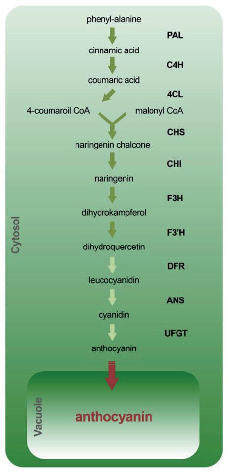
4: Process of Anthocyanin Biosynthesis (Source:

This experiment explores the two most common methods of extracting anthocyanin and determining its concentration within the Purple Heart Plant. The plant

is a long-jointed groundcover plant with pointy, purple leaves as shown below in Figure 5:

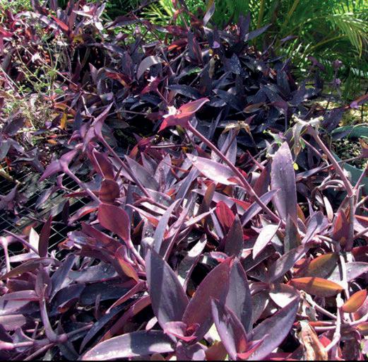
Figure 5: Image of the Purple Heart Plant (tradescantia pallida) (Source: Rojas-Sandoval & Acevedo-Rodríguez, 2013)

Studies have shown that this plant produces more anthocyanin when exposed to a greater light intensity (Paiva et al., 2003), but the effect of UV exposure time has not yet been explored. The first method utilises colourimetry to produce a mathematical relationship capable of predicting anthocyanin content. A chromameter determines L,a,b values for the colour it detects, where ‘L’ is luminousity, ‘a’ is a measurement of how red or green something is, and ‘b’ is a measurement of how blue or yellow something is. L values range from 0 (dark) to 100 (light). The ‘a’ value ranges from -128 (green) to 127 (red), and the ‘b’ value ranges from -128 (blue) to 127 (yellow) (Martin, 2015). As shown in Figure 8a and Figure 8b, these L,a,b values are used to calculate h and C values, where h is the hue and C is the saturation. These five results are crucial to this method of determining anthocyanin. These results can then be combined with experimental data of anthocyanin content in a plant, and a reliable formula can be formed, as shown in the equation:

Equation 1: Chromatic equation for calculating total anthocyanin content (Vieira et al., 2018).

Despite this method, the anthocyanin concentration must be known, so another method is required to produce an accurate formula. Also, the Beta values are coefficients that are formed over a set of data from hundreds of stimuli. Hence, this method was impractical for this experiment, but would remain a useful tool for future experiments.

The second method for determining anthocyanin uses a colourimeter to analyse an absorption value at a particular wavelength. Colourimetry is the science of measuring colours to analyse compounds. (Academy, 2022). This is done via the analysis of the wavelengths and intensity of electromagnetic radiation within the visible spectrum (Colorimetry | Light Measurement, Photometry & Spectrophotometry | Britannica, 2024). The pigments from finely cut plants are dissolved into 70% ethanol. Substances such as ethanol, methanol, and acetone are commonly used to extract anthocyanin (Tena & Asuero, 2022). This new solution is then filtered to remove leaves, then placed into cuvettes. The cuvettes are inserted into the colourimeter, and the resulting absorbance value is determined (Colourimetry - an Overview | ScienceDirect Topics, 2012). Using the absorbance value, Beer-Lambert’s Law allows for the anthocyanin content to be calculated:

Equation 2: Equation 3 - Beer-Lambert's Law

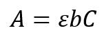
A = Absorbance

ε = Molar Absorptivity

b = Length of light path

C = Concentration

Scientific Research Question

What is the effect of UV light exposure time on the concentration of anthocyanin within tradescantia pallia?

Scientific Hypothesis

As the exposure of UV light time increases, the concentration of anthocyanin within the Purple Heart plant will also increase. However, a critical point will exist where any more exposure is detrimental to anthocyanin accumulation.

Where:

Y = total anthocyanin content

X = independent variables linked to the L,a,b,C,h values

Beta = constants of each independent variable

Methodology

Ten tradescantia pallida plants were selected for this investigation. Two were kept in the original garden whilst another two were transferred into pots without

UV treatment to act as controls and assess if repotting drastically changes the anthocyanin content. The remaining six plants were then exposed to UV light (254nm) for periods of 2, 6 or 12 hours with 2 plants randomly assigned to each time interval. This was done underneath a cover to prevent any outside light from reaching the plant. Following treatment the plants were then rested for 24 hours prior to further analysis.

Leaf samples (5 g) were collected from each of the 10 individual plants. The fresh weight of each sample was recorded, and the colorimetric properties (L*, a*, b* values) were measured using a Minolta CR-200 chromameter. Following measurement, the leaf material was finely chopped using a clean stainless steel knife and transferred into Schott bottles. Samples were grouped based on their respective exposure durations. Each bottle was then filled with 50 mL of 70% ethanol, immediately sealed, and wrapped in aluminium foil to prevent light exposure. The samples were subsequently refrigerated at 4 °C for 24 hours. This procedure was repeated for a second trial set of plants. These plants were left for an additional 24 hours more than the first trial.

The leaf/ethanol mixtures were filtered, isolating the pigment extract. A Pasco Spectrometer was calibrated with a cuvette containing 70% ethanol. The absorbance of each extract solution was measured at 535nm. And the anthocyanin concentration calculated

using Beer Lambert’s Law, which is demonstrated in Equation 2.

Results

The measurements from the Minolta CR200 Chromameter remained mostly consistent within the same groups. For example, the Trial 1 set of 2-hour exposure had very similar measurements but were different to 6-hour samples. However, some outliers existed, presenting colour values far outside the norm. Upon closer inspection, these leaves were also slightly greener as well as just purple. These leaves were discarded in favour of those with similar colours to the other leaves. Using equations 3 and 4, the hue and saturation values were found and added to tables 1 and 2. There was little difference between Trial 1 and Trial 2’s results in this section.

Equation 3: Hue value

Equation 4: Saturation value (Vieira et al., 2018)

Table 2: Trial 2 (Original L,a,b values of leaves + absorbance and concentration 24 hours after Trial 1)

From the data in Table 1 and Table 2, t-tests were run to detect if UV exposure time has a significant impact on the concentration of anthocyanin within the plant.

Table 3: T-test between the means of the two trials

t-Test: Paired Two Sample for Means:

1

Variance 0.027007 2.024489

Observations 4 4

Pearson

Correlation -0.65469

Hypothesized Mean Difference 0

df 3

t Stat -1.91766

P(T<=t) one-tail 0.075493

t Critical one-tail 2.353363

P(T<=t) two-tail 0.150985

t Critical two-tail 3.182446

The t-test has a p value of 0.075493 for one-tail, and 0.150985 for two-tail. For an alpha value of 0.05, the null hypothesis could not be rejected, meaning we cannot determine this to be significant.

After exposing the leaves to 70% ethanol solutions in refrigerated conditions, the now coloured solutions were placed into cuvettes to be analysed within a chromometer. The absorbance value (A) demonstrated a clear relationship with the UV light exposure time. Using two cuvettes for each solution allowed for a more accurate correlation. Strangely, Trial 1 and Trial 2 had major differences in values.

Using the absorbance values, the concentration of anthocyanin was determined for each group using the equation:

Equation 5: Concentration of anthocyanin through absorption (Source: Vieira et al., 2018)

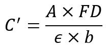
Where:

C’ = Total anthocyanin content (mg/L)

A = Absorbance (535nm)

Epsilon = Absorbance coefficient of cyanidines (98.2)

B = Thickness of the cuvette (1cm)

FD = Dilution Factor of the extract (1 in this experiment)

1)

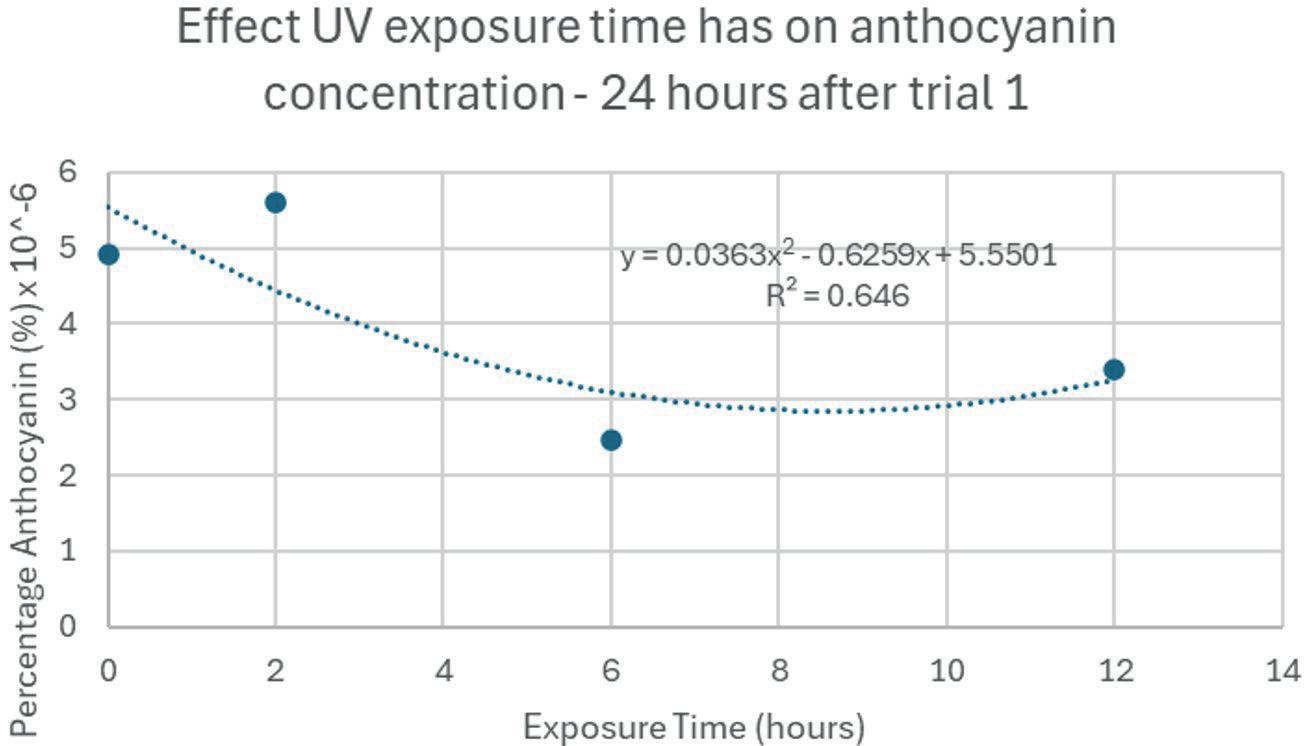
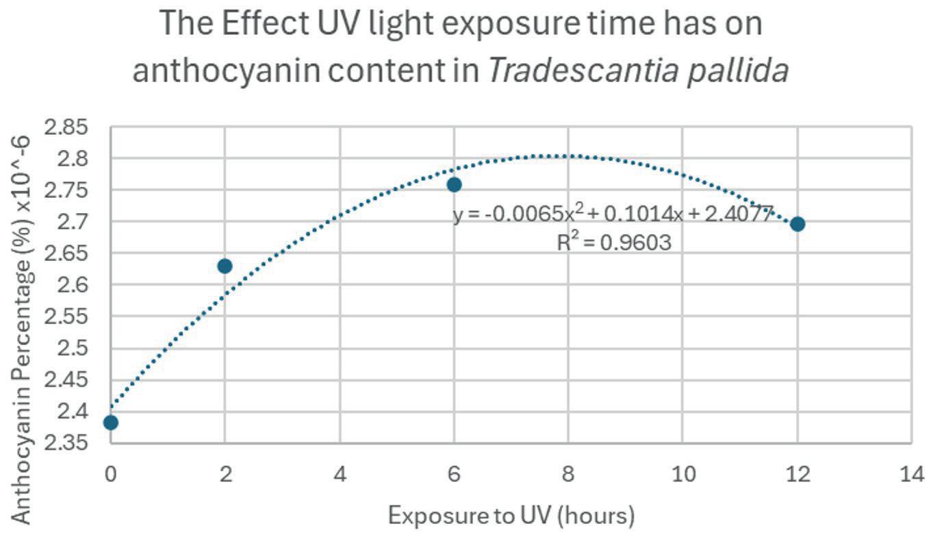
8: Effect of UV light exposure on anthocyanin content (Trial 2)

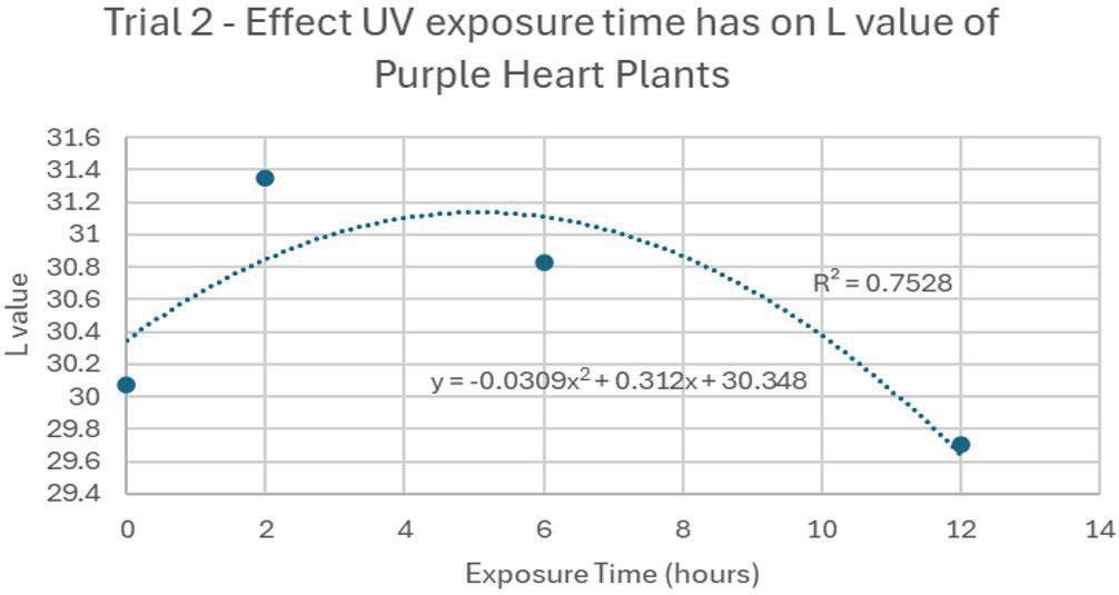
on L value (Trial 2)

Discussion

Despite the results, calculating anthocyanin concentration with the mathematical equation

required several unknown coefficients that could not be found. Hence, anthocyanin could not be calculated using the L,a,b method.

The anthocyanin content was shown to increase with exposure to UV light, but there was a point where any additional exposure resulted in a lower concentration. In Trial 1, the maximum anthocyanin percentage was at 8 hours, where anthocyanin content was 2.8 × 106 %. However, 12 hours had 2 7 × 10 6 %, which is clearly lower. This may have been because the UV light began to damage plant tissue as well as stimulate anthocyanin biosynthesis. This would likely result in the plant focussing on the damaged areas of the leaves rather than producing more anthocyanin. Or the anthocyanin itself broke down, caused directly by the UV. More research should be done to identify which of these possibilities is correct.

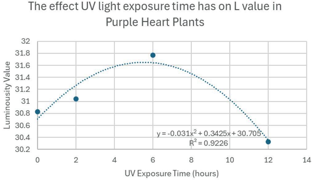
The data from the trials is demonstrated in figures 6a, 6b, 7a, and 7b. Exposure time to UV light had a negative parabolic relationship with the L value, A value, and anthocyanin content. Hence, there is a peak value of UV exposure time to achieve the greatest amount of anthocyanin. As previously stated, the maximum anthocyanin percentage was at 8 hours, where anthocyanin content was 2 8 × 106 %. The content with no additional UV exposure yielded 2 4 × 10 6 %. This means that the exposure to UV increased anthocyanin content by 14 percent.

For the L value, the colour of the leaves were the brightest around 5-6 hours, before becoming darker again. The a value had a relatively flat relationship, suggesting that the change in UV light exposure time had only a small effect on the red and green components of the colour. The B and H values both had positive quadratic relationships. The B value was lowest around 6 hours, suggesting that exposing the plant to UV for a certain amount of time decreases the blue and yellow contents of the colour. The H value (hue) had a minimum around 3 hours. The C value (saturation) had a negative parabolic relationship with UV exposure time, meaning it became more vibrant until around 6 hours, before becoming duller.

The first and second trials had major differences between the two despite expectations. Since Trial 2 occurred 24 hours after Trial 1, there is a possibility that some of the anthocyanin had converted back into other chemicals for the plant, since the stimulus had long been removed. Also, the percentage anthocyanin within each sample is low compared to experimental data. For example, a peak of 2 8 × 10 6 % when anthocyanin content is normally far higher. Within the

method, the solution is usually diluted for more accurate results. This may be the source of the error. The means of Trial 1 and Trial 2 not being significantly different suggests that an additional 24 hours before analysis did not affect the anthocyanin percentage in a significant way. However, the differences between the relationships in the graphs would suggest otherwise. The experiment should be repeated to test the reproducibility of the results.

A key limitation in this experimental process was the relatively small sample size. A larger sample size and exposure every hour would result in more precise data, leading to an improved relationship. Additionally, having a larger sample size would increase the validity of the results.

UV light has increased noticeably over the past couple of decades (L & Jk, 2012). Further implications from this experiment may be how plants will behave when exposed to a higher level of UV. Plants may experience too much UV light, resulting in anthocyanin breaking down. This would become a problem as our diets would likely contain less antioxidants, which would lead to more free radicals and potentially health problems becoming more common.

Conclusion

This experiment investigated the effect exposure time to UV light has on the resulting accumulation of anthocyanin in tradescantia pallida. The results of Trial 1 demonstrated the expected negative parabolic relationship, but was not reproduced in a second trial. As exposure time lengthened, anthocyanin content initially increased to a maximum. However, a critical time was reached, where any more exposure to UV was detrimental to both anthocyanin content and the overall health of the plant. Additionally, a t-test was utilised to identify if there was any significant difference between the means of the two trials. The results did not determine any significant difference between the two means. Hence, leaving the plant for an additional 24 hours before analysis should not majorly affect the anthocyanin content. However, it is unclear as to why a positive parabolic relationship would exist between the exposure time and the anthocyanin concentration within the second trial. More experimentation should be completed to confirm this as correct result.

In Trial 1, 8 hours of UV light maximised the anthocyanin content to 2 8 × 10 6 %. However, any more exposure resulted in a decrease in content. For

example, 12 hours of exposure yielded 2 7 × 10 6 % anthocyanin.

The main limitation with the experiment was the low sample size. Two cuvettes for each absorption reading is inadequate for a more thorough understanding of the relationship between UV exposure time and anthocyanin accumulation. Also, the cuvettes may have had small smudges, which would lead to more inaccurate results.

More experimentation should be done to identify the exact peak exposure time resulting in the most anthocyanin, as every plant likely has a different preference of exposure time. This phenomenon should also be explored, testing other plants to find any common patterns between species. The link between UV exposure and the daylight cycle should also be explored for this plant.

Acknowledgements

I would like to thank Mrs Kathy Haigh for her invaluable assistance in this experiment. She guided me throughout the process of experimentation, such as her providing a Science Research laboratory at the school to undertake the method.

References

Academy, V. S. (2022, August 31). Colorimetry Vision Science Academy https://visionscienceacademy.org/colourimetry/

Arnarson, A. (2023, July 12). Antioxidants Explained in Simple Terms. Healthline. https://www.healthline.com/nutrition/antioxidantsexplained

Colorimetry | Light Measurement, Photometry & Spectrophotometry | Britannica. (2024, October 17). https://www.britannica.com/science/colorimetry

Dong, W., Yang, X., Zhang, N., Chen, P., Sun, J., Harnly, J. M., & Zhang, M. (2024). Study of UV–Vis molar absorptivity variation and quantitation of anthocyanins using molar relative response factor. Food Chemistry, 444, 138653. https://doi.org/10.1016/j.foodchem.2024.138653

Enaru, B., Drețcanu, G., Pop, T. D., Stǎnilǎ, A., & Diaconeasa, Z. (2021). Anthocyanins: Factors Affecting Their Stability and Degradation. Antioxidants, 10(12), 1967. https://doi.org/10.3390/antiox10121967

Goodman, T. (2012). Colourimetry An overview | ScienceDirect Topics https://www.sciencedirect.com/topics/engineering/colouri metry

Holton, T., & Cornish, E. (n.d.). Genetics and Biochemistry of Anthocyanin Biosynthesis PMC. Retrieved November 20, 2024, from https://pmc.ncbi.nlm.nih.gov/articles/PMC160913/

Humans, I. W. G. on the E. of C. R. to. (2012). Solar and ultraviolet radiation. In Radiation. International Agency for

Research on Cancer. https://www.ncbi.nlm.nih.gov/books/NBK304366/

Khoo, H. E., Azlan, A., Tang, S. T., & Lim, S. M. (2017). Anthocyanidins and anthocyanins: Colored pigments as food, pharmaceutical ingredients, and the potential health benefits. Food & Nutrition Research, 61(1), 1361779. https://doi.org/10.1080/16546628.2017.1361779

L, L.-D., & Jk, M. (2012). Fifty years of changes in UV Index and implications for skin cancer in Australia. International Journal of Biometeorology, 56(4). https://doi.org/10.1007/s00484-011-0474-x

Lubeck, B. (2024, September 3). What Are Anthocyanins? Verywell Health. https://www.verywellhealth.com/anthocyanins-benefits89522

Martin, A. (2015). 4.4 Lab Colour Space and Delta E Measurements

https://opentextbc.ca/graphicdesign/chapter/4-4-lab-colourspace-and-delta-e-measurements/

Mattioli, R., Francioso, A., Mosca, L., & Silva, P. (2020). Anthocyanins: A Comprehensive Review of Their Chemical Properties and Health Effects on Cardiovascular and Neurodegenerative Diseases. Molecules, 25(17), 3809. https://doi.org/10.3390/molecules25173809

Ovando, C. (2009). Anthocyanin An overview | ScienceDirect Topics

https://www.sciencedirect.com/topics/agricultural-andbiological-sciences/anthocyanin

Paiva, É. A. S., Isaias, R. M. dos S., Vale, F. H. A., & Queiroz, C. G. de S. (2003). The influence of light intensity on anatomical structure and pigment contents of Tradescantia pallida (Rose) Hunt. Cv. Purpurea Boom (Commelinaceae) leaves. Brazilian Archives of Biology and Technology, 46, 617–624. https://doi.org/10.1590/S151689132003000400017

Pintér, J., Kósa, E., Hadi, G., Hegyi, Z., Spitkó, T., Tóth, Z., Szigeti, Z., Páldi, E., & Marton, L. (2007). Effect of increased UV-B radiation on the anthocyanin content of maize ( Zea mays L.) leaves https://doi.org/10.1556/AAgr.55.2007.1.2

Pojer, E., Mattivi, F., Johnson, D., & Stockley, C. S. (2013). The Case for Anthocyanin Consumption to Promote Human Health: A Review. Comprehensive Reviews in Food Science and Food Safety, 12(5), 483–508. https://doi.org/10.1111/1541-4337.12024

PubChem. (2025). Flavylium. https://pubchem.ncbi.nlm.nih.gov/compound/145858

Rojas-Sandoval, J., & Acevedo-Rodríguez, P. (2013). Tradescantia pallida (purple queen). CABI Compendium, CABI Compendium, 117574. https://doi.org/10.1079/cabicompendium.117574

Shi, C., & Liu, H. (2021). How plants protect themselves from ultraviolet-B radiation stress. Plant Physiology, 187(3), 1096–1103. https://doi.org/10.1093/plphys/kiab245

Tena, N., & Asuero, A. G. (2022). Up-To-Date Analysis of the Extraction Methods for Anthocyanins: Principles of the Techniques, Optimization, Technical Progress, and Industrial Application. Antioxidants, 11(2), 286. https://doi.org/10.3390/antiox11020286

Vieira, L. M., Marinho, L. M. G., Rocha, J. de C. G., Barros, F. A. R., & Stringheta, P. C. (2018). Chromatic analysis for

predicting anthocyanin content in fruits and vegetables. Food Science and Technology, 39, 415–422. https://doi.org/10.1590/fst.32517

Wei, Z., Yang, H., Shi, J., Duan, Y., Wu, W., Lyu, L., & Li, W. (2023). Effects of Different Light Wavelengths on Fruit Quality and Gene Expression of Anthocyanin Biosynthesis in Blueberry (Vaccinium corymbosm). Cells, 12(9), Article 9. https://doi.org/10.3390/cells12091225

What Are Free Radicals? And Why Should You Care? (2022, July 19). Cleveland Clinic. https://health.clevelandclinic.org/free-radicals.

Wu, J., Liu, W., Yuan, L., Guan, W.-Q., Brennan, C. S., Zhang, Y.-Y., Zhang, J., & Wang, Z.-D. (2017). The influence of postharvest UV-C treatment on anthocyanin biosynthesis in fresh-cut red cabbage. Scientific Reports, 7, 5232. https://doi.org/10.1038/s41598-017-04778-3

Zhao, T., Li, Q., Yan, T., Yu, B., Wang, Q., & Wang, D. (2025). Sugar and anthocyanins: A scientific exploration of sweet signals and natural pigments. Plant Science, 353, 112409. https://doi.org/10.1016/j.plantsci.2025.112409

Effects of Pre-Harvest UV-C Hormesis on Lycopene Production in Tomato Plants

Kevin Sun Barker College

Lycopene, a powerful antioxidant found abundantly in tomatoes, is linked to various health benefits including cardiovascular protection, cancer prevention, and improved metabolic function. This study investigated the effect of preharvest UV-C hormesis on lycopene production in Solanum lycopersicum ("Large Cherry" variety). Six tomato plants were exposed to varying durations of UVC radiation (0, 0.5, 1, 1.5, 3, and 5 hours), and lycopene content was quantified using solvent extraction and colorimetric analysis at 500 nm. The results revealed a biphasic relationship between UV-C exposure time and lycopene concentration, with peak accumulation occurring at 1 hour (0.00577 mg/g). ANOVA testing showed a significant difference between groups (p = 2.08×10-18, Fstat = 470, F-crit = 2.77), indicating that UV-C treatment duration had a clear effect on lycopene synthesis. These findings support the potential of low-dose UV-C as a practical strategy to enhance nutritional quality in tomatoes through controlled stress induction.

Literature Review

Lycopene

Lycopene is a naturally occurring carotenoid pigment responsible for the red and pink hues in various fruits and vegetables, notably tomatoes, watermelons, and pink grapefruits (Rao & Agarwal, 2000). Beyond its role in plant pigmentation, lycopene has garnered attention for its potential health benefits in humans (Story et al., 2010)

Chemical Structure

Chemically, lycopene is a symmetrical tetraterpene hydrocarbon forming a long, linear molecule with 11 conjugated double bonds (alternation between single and double bonds), shown in Figure 1 This extensive conjugation imparts its deep red colour and contributes to its antioxidant properties as long conjugated regions result in the absorption of broader light particles (Cooper & Klymkowsky, 2020)

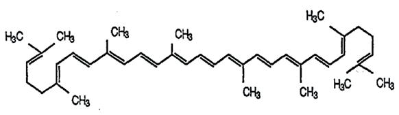
Figure 1: Chemical structure of Lycopene (all-trans configuration) (Source: Cámara et al., 2013)

In nature, lycopene primarily exists in the all-trans configuration, a linear and stable form of the molecule (Boileau et al., 2002). However, when exposed to heat or light, isomerization occurs, converting it into cisisomers, which have a bent structure and may be more

bioavailable meaning they are more easily absorbed by the body (Stahl & Sies, 1996).

Health Benefits

Lycopene is recognized for its potent antioxidant capacity, enabling it to neutralize reactive oxygen species (ROS) (highly reactive molecules containing oxygen created as a byproduct of cellular metabolism) and reduce oxidative stress (occurs when excess ROS causes damage to DNA, protein and cell membrane), a factor implicated in the development of various chronic diseases (Sies, 1997)

Lycopene intake has been associated with improved cardiovascular health, including reductions in blood pressure and the inhibition of angiotensin-converting enzyme activity, which plays a key role in blood pressure regulation (Bin-Jumah et al., 2022) Additionally, cancer prevention has been linked to lycopene, with some studies suggesting it may help manage or reduce the risk of certain cancers such as prostate and pancreatic cancer by decreasing oxidative stress and influencing gene expression (P. D. Sarkar et al., 2012). Lycopene intake has also shown promise in supporting metabolic health, with evidence indicating its potential to aid in the management of conditions like obesity and type 2 diabetes mellitus, primarily due to its antioxidant and anti-inflammatory properties (Leh & Lee, 2022)

While raw tomatoes and other red fruits contain mostly all-trans lycopene, cooking and processing increase the proportion of cis-isomers, which could enhance their potential health benefits (Rao & Agarwal, 2000). Although research shows that

lycopene can attenuate a wide range of chronic conditions, how lycopene exerts this bioactivity remains relatively unknown (Arballo et al., 2021)

Biosynthesis in Plants

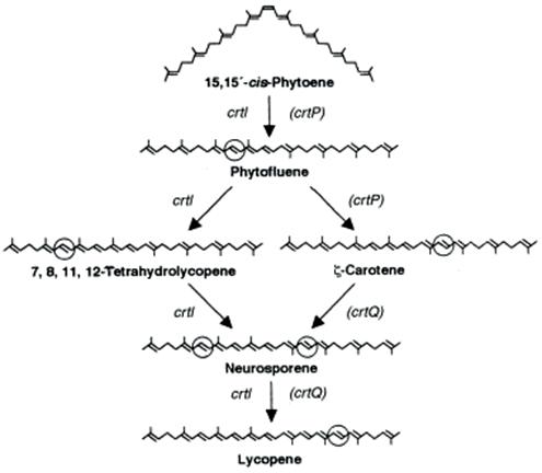
In photosynthetic organisms, lycopene serves as an intermediate in the biosynthesis of various carotenoids (Cunningham & Gantt, 1998). The biosynthetic pathway begins with the condensation of two molecules of geranylgeranyl pyrophosphate (GGPP), a 20-carbon molecule that serves as a building block for carotenoids, to form phytoene, a colourless carotenoid (A class of naturally occurring pigments, including Lycopene) in the plastids, which are the main sites of photosynthesis in eukaryotic cells (Fraser & Bramley, 2004). Phytoene then undergoes a series of desaturation (process in which two hydrogen bonds are removed to more double bonds) and isomerization reactions to form lycopene, as seen in Figure 2. These reactions, enabled by gene encoding enzymes phytoene desaturase (crtI), ζ-carotene desaturase (crtQ), and phytoene dehydrogenase (crtP), introduce conjugated double bonds into the molecule, transforming the colourless phytoene into the deep-red lycopene.

Regulation of Lycopene Biosynthesis

The accumulation of lycopene in plant tissues is regulated by various factors. Gene expression plays a crucial role in lycopene production, as transcriptional regulators proteins or small molecules that bind to DNA can activate or repress carotenoid biosynthetic genes in response to external stimuli (Fraser & Bramley, 2004). Through the process of hormesis, in which exposure to a low dose of a typically harmful agent induces a beneficial adaptive response, lycopene synthesis may be enhanced. Environmental factors such as light exposure and temperature also influence

lycopene levels by affecting the activity of key enzymes within the carotenoid biosynthesis pathway. In addition, hormonal control, particularly through plant hormones like ethylene, is vital during the ripening process, a stage in which lycopene accumulation is significantly increased in fruits such as tomatoes (Stanley & Yuan, 2019)

UV-C Hormesis

UV-C hormesis is a phenomenon in which low, nonlethal doses of UV-C radiation (the shortest and most harmful wavelength of UV) stimulate beneficial responses in plants, enhancing their health, growth, and resistance to environmental stress (Volkova et al., 2022). The key mechanism behind this effect is the controlled generation of reactive oxygen species (ROS) such as superoxide anions (O₂⁻) and hydrogen peroxide (H₂O₂). While excessive ROS production at high UV-C doses can cause oxidative stress and cellular damage, low doses trigger signalling pathways that activate antioxidant defence and stresstolerance genes. These include genes responsible for antioxidant enzymes like superoxide dismutase and catalase, as well as heat shock proteins and phytoalexins, which act as natural antimicrobial compounds. For instance, a study on lettuce seedlings treated with UV-C demonstrated a significant decrease in disease severity when challenged with the pathogen Xanthomonas campestris. Transcriptomic analysis revealed the upregulation of genes involved in various defence pathways, suggesting that UV-C treatment primes the plant's immune system to respond more effectively to pathogens (Sidibé et al., 2022a)

Another important benefit of UV-C hormesis is the increased production of phytochemicals such as flavonoids, phenolic acids, and anthocyanins. These secondary metabolites play key roles in UV protection, antioxidant activity, and overall plant health. For example, flavonoids absorb UV radiation, shielding plant tissues from damage, while also acting as antioxidants to neutralize harmful ROS. Research has shown that UV-C exposure enhances the concentration of these compounds in crops like tomatoes and lettuce, improving both their nutritional value and resistance to spoilage (Loconsole & Santamaria, 2021). Additionally, UV-C exposure helps delay senescence, or plant aging, by maintaining chlorophyll content and stabilizing cellular structures. This effect extends the productive lifespan of crops and has practical applications in postharvest storage by slowing down deterioration and prolonging freshness (Lemoine et al., 2007)

The effectiveness of UV-C hormesis follows a biphasic dose-response curve Figure 3, meaning that low doses lead to positive effects such as improved growth, increased disease resistance, and higher phytochemical production. Meanwhile, higher doses can be detrimental, causing DNA damage, cellular stress, and reduced plant viability (Correa et al., 2023) This makes it crucial to determine the optimal UV-C dose for each plant species. However, the exact optimal UV-C amount for lycopene in tomatoes contains a literature gap. In agricultural applications, UV-C hormesis has been used to enhance disease resistance and reduce the need for chemical pesticides. Preharvest UV-C treatments, for instance, have been found to decrease fungal infections such as Botrytis cinerea in tomatoes, while postharvest treatments have increased the amounts of antioxidants and bioactive compounds (Bravo et al., 2012).

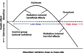
Figure 3: Biphasic dose-response model on hormetic radiation (Source: Cuttler et al., 2021)

Lycopene extraction

Due to its non-polar and lipophilic nature (hydrophobic), lycopene is typically extracted using organic solvents such as hexane, ethanol, acetone, or their mixtures (Periago et al., 2004). After thorough mixing, water is added to separate the solution into layers, with lycopene collecting in the upper organic phase. This layer is then removed, filtered, and may be analysed using spectrophotometry or HPLC to quantify lycopene content. The method chosen was derived from (Anthon & Barrett, 2007) using a hexane:acetone:ethanol mixture and ice to reduce thermal degradation.

Colourimetry

A colorimeter functions by directing a specific wavelength of light through a solution containing a compound capable of absorbing that light. As the light passes through the sample, a portion is absorbed, and the remaining light is measured by a detector on the opposite side. In colorimetry, measurements are usually taken at the λmax (maximum light absorbance) of the measured substance, ensuring maximum sensitivity and accuracy (Choudhury, 2014)

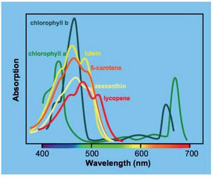
Figure 4: Light absorbance of various carotenoids and pigments found within tomatoes

As seen in Figure 4, other pigments and carotenoids found in tomatoes such as β-carotene and chlorophyll also have high absorbance values at 471 nm (λmax), thus causing interference from other compounds and affecting the accuracy of the readings. 503 nm was chosen because, while not the absolute maximum absorbance of lycopene, it offers greater specificity by minimizing interference from other carotenoids and provides a broader, more stable peak for consistent quantification in complex mixtures.

According to the Beer-Lambert Law (Equation 1), the amount of light absorbed is directly proportional to the concentration of the absorbing compound. Based on prior research, lycopene exhibits optimal absorbance at a wavelength of 503 nm (Amorim et al., 2022).

Equation 1: Beer Lambert's Law

�������� = �������� × �������� × ��������

Where

�������� = absorbance

�������� = molar absorptivity

�������� = optical path length

�������� = concentration

Scientific Research Question

How will preharvest UV-C hormesis affect the lycopene production in tomato plants at various exposure levels?

Scientific Hypothesis

There will be a biphasic relationship between the level of UV-C exposure and the amount of lycopene produced in tomatoes, where lycopene levels will increase as low-doses of UV-C hormesis are utilised

until a certain point where higher doses will have detrimental effects on lycopene production.

Methodology

Tomato samples and UV-C treatment

Six tomato plants (Solanum lycopersicum, "Large Cherry" variety) were grown concurrently to ensure environmental factors had minimal effect on lycopene variation within batches, starting from the budding stage in an outdoor open environment. The plants were maintained under optimal agronomic conditions, including regular irrigation, fertilization, and pest management, until they reached the mature green (breaker) stage.

At the breaker stage, marking the first signs of ripening, the plants were moved indoors to ensure optimal UV-C absorption and were subjected to hormetic UV-C treatment under 5 different conditions and one control group. The five test plants were irradiated under ambient conditions using an 8W UVC lamp with a peak wavelength of 254 nm. The UVC chamber measured 55 cm wide, 55 cm deep, and 97 cm high, containing an 8W lamp that emitted UV-C light. The chamber was then completely covered with dark cloth to reduce external light exposure, minimising uncontrolled variables. The plants were irradiated with UV-C continuously for either 0.5, 1, 1.5, 3 and 5 hrs, with each condition being assigned a random plant. After hormetic treatment of the five plants, the tomatoes from all six plants were allowed to ripen on the vine under day/night cycle illumination conditions at room temperature for up to 10 days. During the 10 days of ripening, tomatoes were harvested when they turned red and immediately frozen. After the 10 days, each group of tomatoes were then cut up using a knife, homogenized using a mortar and pestle, and stored under freezing conditions until analysis.

Lycopene Extraction

Approximately 2 g (determined to the nearest 0.01 g) from each group, including the control, were weighed from the samples into six 100 ml amber screw-top vials containing 16.5 ml of acetone, 16.5 ml of 95% USP grade ethanol, and 33 ml of hexane. Each sample was then thoroughly mixed and extracted on an orbital shaker at 180 RPM for 15 minutes on ice to prevent thermal degradation. After shaking, 5 ml of deionized water, used to prevent contamination, were added to each vial, and the samples were shaken for an additional 5 minutes on ice. The vials were then left at room temperature for 5 minutes to allow for phase separation.

Lycopene Analysation

A PASCO colourimeter was used alongside SPARKvue data logging software. A sample of the hexane:ethanol:acetone solvent mixture was placed into a clean quartz cuvette and used to calibrate the colourimeter at 500nm. The coloured organic layer from each volumetric flask was then used to fill a clean and dry disposable cuvette and absorbance at 500 nm was recorded. Due to the potential for solventinduced degradation (such as microfracturing or "crazing") of the cuvette surface, measurements were taken as quickly as possible to ensure accuracy. Each sample was measured four times to check reliability and reduce the impact of random errors on the results. The absorbance values of the samples were then converted into mg/g tissue using the following equation:

Equation 2: converts the raw absorbance values into lycopene (mg) per g of sample using values derived from (Sahoo et al., 2013)

Results

The results are displayed through two tables showing the raw values of absorbance (Table 1) and concentration of lycopene (Table 2). Figure 5 graphs the average concentration of lycopene across the six consecutive levels of UV-C irradiance. Finally, the results of an ANOVA with post hoc Tukey HSC tests are displayed in Tables 3 and 4.

Table 1: Absorbance values (3 Sig Fig) of each sample

Table 2: Concentration of Lycopene (3 Sig Fig) in each sample

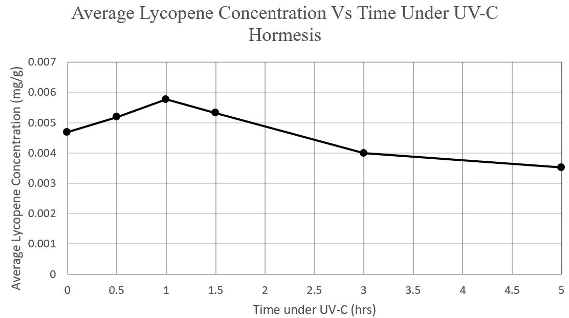
Figure 5: Line graph showing the relationship between average lycopene concentration and time under UV-C

Table 3: Descriptive statistics and ANOVA test results for sample concentrations

Table 4: Tukey HSD test results. Grey rows indicate a significant difference between groups.

P-Value = 2.08 x10-18

F-Statistic = 470

F-Critical = 2.77

The results of the ANOVA reveal there is a significant difference in means between at least two of the groups (p=2.0 x10-18).

The results of the post hoc Tukey HSD test revealed that all means were significantly different with the exception of times of 0.5 and 1.5 hours of UV-C irradiation. However, it is important to note that 0.5 and 1.5 hours are not consecutive groups (see Figure 5) and the mean at 0.5 hour is significantly different from the higher mean at 1 hour (p=4.595 x10-8) and the mean at 1 is significantly different from the lower mean at 1.5 hours (p=0.000003274). The means of each consecutive group are significantly different.

Discussion

The results of this investigation support the hypothesis that low doses of preharvest UV-C exposure stimulate lycopene accumulation in tomatoes, and that this effect diminishes and reverses at higher doses forming a biphasic (parabolic-like) response with a peak (Figure 5). The results of the ANOVA (Table 3) with post hoc Tukey HSD tests (Table 4: Tukey HSD test results. Grey rows indicate a significant difference between groups. confirmed that there were significant differences between groups (p=2.08 x10-18) specifically, that the means at each consecutive time were significantly different from each other. The peak average lycopene concentration (0.00577 mg/g) was observed after 1 hour of UV-C exposure, where the lycopene extracted was 23.3% more than the control group at 0.00468mg/g (Table 2). Moreover, reduced

concentrations were recorded at both lower and higher durations (Figure 5: Line graph showing the relationship between average lycopene concentration and time under UV-C.

The trend observed where lycopene levels increase at 0.5–1 hour of UV-C exposure but decrease at 1.5–5 hours is biologically consistent with previous findings on hormetic responses in plants (Sidibé et al., 2022b). The initial increase may result from UV-Cinduced activation of transcriptional regulators in the carotenoid biosynthetic pathway, enhancing lycopene synthesis. However, prolonged exposure likely leads to oxidative stress, cellular damage, or degradation of lycopene itself, resulting in reduced concentrations (Ribaya-Mercado et al., 1995)

Two key sources of systematic error may have affected the accuracy of lycopene quantification in this experiment. Firstly, absorbance measurements were taken at 500 nm rather than the optimal 503 nm (Amorim et al., 2022), due to limitations in the school laboratory and the unavailability of a more precise colorimeter. While this likely resulted in a consistent underestimation of lycopene concentration, it did not compromise the validity of the overall trend, as all samples were measured under the same conditions. Secondly, butylated hydroxytoluene (BHT), a stabilising antioxidant that helps prevent oxidative degradation of lycopene during extraction (Choudhari & Ananthanarayan, 2007), was not used. This was due to restricted access to chemical reagents in a school lab setting. As a result, some degradation may have occurred, particularly when samples were exposed to light or air. However, since both of these factors are systematic in nature affecting all samples consistently they do not impact the comparative relationships observed between treatments.

Lastly, one potential source of error in this experiment arises from the distribution of lycopene within the tomato fruit. According to (S. Sarkar et al., 2013), the outer epidermis of the tomato contains the highest concentration of lycopene. This presents a methodological limitation, as the homogenization process may not have ensured a consistent ratio of skin to pulp across all samples. Slight differences in the proportion of epidermis included in each homogenized sample could lead to inconsistent lycopene concentrations, independent of the UV-C treatment effects. Additionally, as tomato size increases, the surface area increases at a slower rate than the volume, resulting in a lower surface area-tovolume ratio in larger tomatoes. This means that smaller tomatoes, which contain a higher proportion of skin relative to flesh, might appear to have higher

lycopene concentrations if more epidermis is included in the sample, potentially skewing results. However, due to the use of a small cherry tomato variety, which exhibits relatively uniform size and high surface areato-volume ratios across fruits, tomato size is not a factor that would have significantly impacted the results in this study.

Future work

To improve the reliability and accuracy of this investigation, several methodological refinements could be made. Firstly, increasing the sample size beyond one plant per treatment group would help capture a broader range of biological variability and strengthen the statistical power of the results. Secondly, while a PASCO colourimeter provided sufficient resolution for preliminary analysis, future studies should consider using higher-resolution spectrophotometers or HPLC (High-Performance Liquid Chromatography) to precisely isolate and quantify lycopene, eliminating potential interference from other carotenoids such as β-carotene or chlorophyll.

This investigation also raises new questions worth exploring. For instance, would postharvest UV-C treatment result in similar or enhanced lycopene accumulation? Could combinations of UV-C and other environmental stressors such as heat, drought, or nutrient variation produce synergistic effects? Moreover, understanding the impact of preharvest UV-C treatment on other aspects of tomato quality, such as flavour, texture, or shelf life, could broaden the practical relevance of this research in agricultural and commercial contexts. Future investigations along these lines would help refine UV-C hormesis as a strategy for enhancing the nutritional value of tomatoes and contribute to broader developments in sustainable crop management.

Conclusion

This study demonstrated that preharvest UV-C hormesis significantly affects lycopene production in tomatoes, with low doses promoting lycopene synthesis and higher doses reducing it. The results align with the proposed hypothesis of a biphasic relationship between time under UV-C and lycopene concentration, and differences between means (excluding 0.5 hrs and 1.5 hrs) were confirmed with an ANOVA (p=2.08 x10-18) and a Tukey HSD test. The optimal exposure was identified at 1 hour, after which lycopene concentration declined, likely due to oxidative damage or metabolic suppression. These findings contribute to the growing body of research supporting hormesis as a valuable tool in agricultural

biotechnology for enhancing crop nutritional value. Future studies using more precise quantification methods such as HPLC and a larger sample size could further validate and refine this approach.

Acknowledgements

I would like to thank Mrs Kathy Haigh for helping with the preparation and execution of the experiment. I would also like to thank Dr Mattew Hill for providing formatting and statistical analysis assistance on this paper.

References

Amorim, A. das G. N., Vasconcelos, A. G., Souza, J., Oliveira, A., Gullón, B., de Souza de Almeida Leite, J. R., & Pintado, M. (2022). Bio-Availability, Anticancer Potential, and Chemical Data of Lycopene: An Overview and Technological Prospecting. Antioxidants, 11(2), 360. https://doi.org/10.3390/antiox11020360

Anthon, G., & Barrett, D. M. (2007). Standardization of a rapid spectrophotometric method for lycopene analysis | International Society for Horticultural Science http://www.actahort.org/books/758/758_12.htm

Arballo, J., Amengual, J., & Erdman, J. W. (2021). Lycopene: A Critical Review of Digestion, Absorption, Metabolism, and Excretion. Antioxidants, 10(3), 342. https://doi.org/10.3390/antiox10030342

Bin-Jumah, M. N., Nadeem, M. S., Gilani, S. J., Mubeen, B., Ullah, I., Alzarea, S. I., Ghoneim, M. M., Alshehri, S., Al-Abbasi, F. A., & Kazmi, I. (2022). Lycopene: A Natural Arsenal in the War against Oxidative Stress and Cardiovascular Diseases. Antioxidants, 11(2), Article 2. https://doi.org/10.3390/antiox11020232

Boileau, T. W.-M., Boileau, A. C., & Erdman, J. W. (2002). Bioavailability of all-trans and cis-isomers of lycopene. Experimental Biology and Medicine (Maywood, N.J.), 227(10), 914–919. https://doi.org/10.1177/153537020222701012

Bravo, S., García-Alonso, J., Martín-Pozuelo, G., Gómez, V., Santaella, M., Navarro-González, I., & Periago, M. J. (2012). The influence of post-harvest UV-C hormesis on lycopene, β-carotene, and phenolic content and antioxidant activity of breaker tomatoes. Food Research International, 49(1), 296–302.

https://doi.org/10.1016/j.foodres.2012.07.018

Cámara, M., de Cortes Sánchez-Mata, M., Fernández-Ruiz, V., Cámara, R. M., Manzoor, S., & Caceres, J. O. (2013). Chapter 11 - Lycopene: A Review of Chemical and Biological Activity Related to Beneficial Health Effects. In Atta-ur-Rahman (Ed.), Studies in Natural Products Chemistry (Vol. 40, pp. 383–426). Elsevier. https://doi.org/10.1016/B978-0-444-59603-1.00011-4

Choudhari, S. M., & Ananthanarayan, L. (2007). Enzyme aided extraction of lycopene from tomato tissues. Food Chemistry, 102(1), 77–81.

https://doi.org/10.1016/j.foodchem.2006.04.031

Choudhury, A. K. R. (2014). 6 Colour measurement instruments. In A. K. R. Choudhury (Ed.), Principles of Colour and Appearance Measurement (pp. 221–269).

Woodhead Publishing. https://doi.org/10.1533/9780857099242.221

Cooper, M. M., & Klymkowsky, M. W. (2020). Chapter 2: Spectroscopy: how we know what we know about the structure of matter https://openbooks.lib.msu.edu/oclue/chapter/chapter-2spectroscopy-how-we-know-what-we-know-about-thestructure-of-matter/

Correa, M. del S. S., Saavedra, M. el R. R., Parra, E. A. E., Ontiveros, E. N., Flores, J. del C. B., Montiel, J. G. O., Contreras, J. E. C., Urrutia, E. L., Acevedo, J. G. Á., Nopala, G. E. J., González, A. M. E., Correa, M. del S. S., Saavedra, M. el R. R., Parra, E. A. E., Ontiveros, E. N., Flores, J. del C. B., Montiel, J. G. O., Contreras, J. E. C., Urrutia, E. L., … González, A. M. E. (2023). Ultraviolet Radiation and Its Effects on Plants. In Abiotic Stress in Plants Adaptations to Climate Change. IntechOpen. https://doi.org/10.5772/intechopen.109474

Cunningham, F. X., & Gantt, E. (1998). GENES AND ENZYMES OF CAROTENOID BIOSYNTHESIS IN PLANTS. Annual Review of Plant Physiology and Plant Molecular Biology, 49, 557–583. https://doi.org/10.1146/annurev.arplant.49.1.557

Cuttler, J., Abdellah, E., Goldberg, Y., & Al-Shamaa, S. (2021, February). (PDF) Low Doses of Ionizing Radiation as a Treatment for Alzheimer’s Disease: A Pilot Study ResearchGate. https://www.researchgate.net/publication/350788259_Low _Doses_of_Ionizing_Radiation_as_a_Treatment_for_Alzh eimer's_Disease_A_Pilot_Study

Fraser, P. D., & Bramley, P. M. (2004). The biosynthesis and nutritional uses of carotenoids. Progress in Lipid Research, 43(3), 228–265. https://doi.org/10.1016/j.plipres.2003.10.002

Honda, M. (2022). Chapter 16 - Cyanobacterial and commercially important carotenoids: Biosynthesis, metabolic engineering, biological activities, applications, and processing. In H. Kageyama & R. Waditee-Sirisattha (Eds.), Cyanobacterial Physiology (pp. 211–233). Academic Press. https://doi.org/10.1016/B978-0-32396106-6.00005-8

Leh, H. E., & Lee, L. K. (2022). Lycopene: A Potent Antioxidant for the Amelioration of Type II Diabetes Mellitus. Molecules (Basel, Switzerland), 27(7), 2335. https://doi.org/10.3390/molecules27072335

Lemoine, M. L., Civello, P. M., Martínez, G. A., & Chaves, A. R. (2007). Influence of postharvest UV-C treatment on refrigerated storage of minimally processed broccoli (Brassica oleracea var. Italica). Journal of the Science of Food and Agriculture, 87(6), 1132–1139. https://doi.org/10.1002/jsfa.2826

Loconsole, D., & Santamaria, P. (2021). UV Lighting in Horticulture: A Sustainable Tool for Improving Production Quality and Food Safety. Horticulturae, 7(1), Article 1. https://doi.org/10.3390/horticulturae7010009

Periago, M. J., Rincón, F., Agüera, M. D., & Ros, G. (2004). Mixture Approach for Optimizing Lycopene Extraction from Tomato and Tomato Products. Journal of Agricultural and Food Chemistry, 52(19), 5796–5802. https://doi.org/10.1021/jf049345h

Rao, A. V., & Agarwal, S. (2000). Role of antioxidant lycopene in cancer and heart disease. Journal of the

Exposure Duration

Table 2: Data from the tensile testing of the PLA samples

Ultimate Tensile Strength for PLA Samples (MPa)

Table 3: Data from the tensile testing of the HIPS samples

Tensile Strength for HIPS Samples (MPa)

Table 4: Data from the tensile testing of the nylon samples Exposure

Ultimate Tensile Strength for Nylon Samples (MPa)

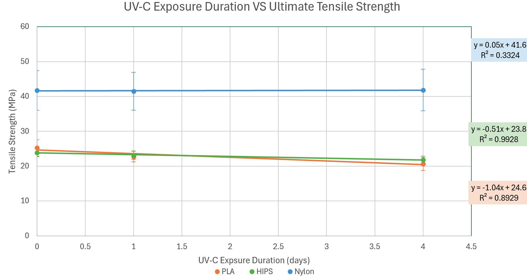
Figure 11: A scatter graph of UV-C exposure duration against the average force of ultimate tensile strength for each polymer, with a line of best fit for each polymer. No x error bands are present as the difference in error for them would be 6.94*10-4 of a day, as the maximum error for extra or less exposure duration is 1 minute.

To compare overall ultimate tensile strength, Figure 11 graphs the ultimate tensile strength of the three polymers tested and includes a linear regression model to show the results of testing.

From the 0-day and 4-day error bars, the potential gradients for PLA range between -1.52 and -0.56, the potential gradients for HIPS range between -0.77 and -0.25 and nylon’s potential gradients range between1.45 to 1.55.

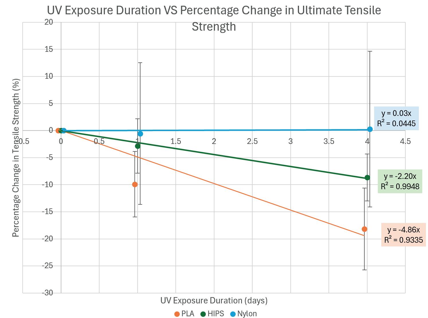
Figure 122: A scatter graph of UV-C exposure duration against the percentage change of ultimate tensile strength from 0 days exposure for each polymer, with a line of best fit for each polymer. The line of best fit for each polymer was forced through the origin, as it is a known point for any percentage change. The same idea was applied to not showing any error bands for the 0-day exposure duration. Note that the points on the graph are for the nearest day, as they were shifted to convey error bands more clearly. No x error bands are present as the difference in error for them would be 6.94*10-4 of a day.

To compare the impact of UV-C exposure on each polymer, Figure 12 plots the percentage change of each polymer. The steeper the regression line, the more the polymer is affected by the duration of UV-C radiation. If a line is flat, there is minimal impact.

As per Figure 11, prior to UV-C exposure, nylon had the highest ultimate tensile strength of 41.7 MPa, and HIPS and PLA had a lower, but similar, initial ultimate tensile strength of 23.9 MPa and 25.2 MPa, respectively. Figure 12 is more useful in showing the impact of UV-C exposure. UV-C exposure had minimal effect on nylon (coefficient of regression = 0.03), a large effect on PLA (coefficient = -4.86, with a reduction in ultimate tensile strength of 18%) and a moderate effect on HIPS (coefficient = -2.20, with a reduction in ultimate tensile strength of 8.7%).

From the 1-day and 4-day error bars for the percentage change graph, the potential gradients for PLA range between -6.76 and -2.96, the potential gradients for HIPS range between -3.23 and -1.13 and nylon’s potential gradients range between -3.47 to 3.53.

Tables 5 and 6 display the results of a one-way ANOVA with post-hoc Tukey tests to determine the significance of the percentage reduction in ultimate tensile strength after four days.

Table 5: Results from the percentage change of each 4-day trial from the 0-day average for each polymer, which was entered into a one-way ANOVA test.

One way ANOVA of the % change of 4-day exposure from 0-day average

Table 6: Post-hoc Tukey tests comparing the differences in percentage reduction for each polymer

Polymer Pairs Q Statistic P Value Inference

PLA vs HIPS 2.96 0.10997 Insignificant

PLA vs Nylon 5.73 0.00108 Significant

HIPS vs Nylon 2.77 0.14162 Insignificant

Discussion

The results from the experiment provide partial evidence supporting the first hypothesis. The PLA and HIPS polymers both showed a decrease in ultimate tensile strength as UV-C exposure duration increased. However, nylon’s ultimate tensile strength did not change, thus, the first hypothesis is partially supported. The gradients of the graph in Figure 12 appeared to support the second hypothesis, whereby PLA incurred the most loss in ultimate tensile strength, then HIPS, then nylon, due to UV-C exposure. However, the results from the one-way ANOVA test (Table 5 and Table 6) found that there is only a significant difference in the data between PLA and nylon (p = 0.00108). thus, the second hypothesis is only supported for PLA and nylon. This means there was not enough evidence to confirm or reject the second hypothesis when comparing HIPS to the other two polymers, but there is a strong indication that HIPS lost more ultimate tensile strength than nylon. This is supported by the error band of Figure 12 as all the HIPS bands are encompassed by the nylon bands, and most of the HIPS bands are encompassed by the PLA bands.

PLA

Out of the three polymers, PLA showed the greatest percentage change in ultimate tensile strength, with it having the steepest gradient of -4.86 from Figure 12 Compared to the results from (Amza et al., 2021) of a 9% decrease in ultimate tensile strength after 24 hours of UV-C exposure, the line of best fit depicts a percentage change that is 4% less for 24 hours; however, the data point for 1 day is -9.9%, which is closer to prior results (Amza et al., 2021). This signifies that the amount of degradation that can occur from UV-C may not continue to increase as the exposure duration increases beyond four days. The degradation that occurred is likely due to photooxidation of the polymer (due to it containing a Carbon double-bonded to an Oxygen), creating radicals that bond to oxygen, reducing the total bonds of the sample.

Compared to the other two polymers, PLA had a unique break pattern as it broke at the same spot for every sample. When examining the PLA samples,

they had a slight defect from 3D printing, which meant that they broke at a lower tensile force than expected. However, the experiment remained valid despite the irregular pattern of breaking due to the UV-C dose on each point on the sample being the same, and each sample of PLA having the same defect. This means that the bonds broken in the PLA samples still experienced the same amount of UV-C exposure as the HIPS and nylon samples.

When observing the PLA samples post 4 days of UVC exposure, there was a thin layer of powder that was not present in 0-day and 1-day exposure durations. This signifies that enough bonds inside the polymer were broken to form a residue that was no longer connected to the samples, signifying that UV-C radiation was able to break the bonds within PLA.

HIPS

HIPS showed a moderate decrease in ultimate tensile strength, as shown in the percentage change graph (Figure 12), displaying a gradient of -2.20. This signifies that some degradation occurred, which contrasts with the results from (Beninia et al., 2011) This is likely due to the UV globe used in this experiment containing UV-C, which has higher energy photons, as well as the globe having a power of 8W instead of 0.76W. The degradation that occurred is likely to be attributed to the photooxidation of the saturated carbon bond present in HIPS.

Although no detector system was used to try to detect volatile formation from the UV-C radiation acting on HIPS, the formation of volatiles, as seen in (Yuzawa et al., 2013) experiment would explain the decrease in ultimate tensile strength that was found after the exposure of HIPS to UV-C. Furthermore, the weakness of the saturated carbon-carbon bonds likely broke, forming radicals, which resulted in a deterioration of the ultimate tensile strength in HIPS.

There was also a white powder present on the surface of the HIPS polymer after a 4-day exposure duration, which was not present in the 0-day and 1-day exposure durations. This suggests that enough bonds were broken to allow part of the polymer to degrade from the sample, which supports the reduction in the ultimate tensile strength of the 4-day samples.

Nylon

The error bands of Nylon are too wide to determine if there was an increase or decrease in ultimate tensile strength after UV-C exposure. The gradient line of best fit for nylon from Figure 12 had the potential to range from -3.47 to 3.53, which is too large to

determine a notable trend as the actual gradient obtained was almost flat (0.03).

The results from (Wady et al., 2020), which showed there was no decrease in ultimate tensile strength under gamma radiation, which has higher energy photons than UV-C, meaning gamma radiation has a higher capacity to degrade compared to UV-C. This can only be used to support the observation that there was no powder present on any of the nylon samples, signifying that not enough bonds were broken for a substantial part of the polymer to break off.

One-Way ANOVA Test

Per the results of the one-way Anova test conducted with the results in Table 5 and Table 6 there is a significant difference in percentage change of ultimate tensile strength between PLA and nylon, due to the pvalue for this comparison being 0.00108, thus being less than the alpha value of 0.05. However, the results from the ANOVA test displayed p-values of 0.10997 for PLA vs. HIPS and 0.14162 for HIPS vs. nylon, meaning the null hypothesis for these two comparisons cannot be rejected, and the results are not significantly different.

Future Research

The results from the one-way ANOVA test offer opportunities for further research. For example, using more samples for a 4-day exposure duration may show a significant difference between HIPS and the other polymers in the ANOVA test.

Another option for further research is using more exposure durations, for example, 0.5, 2 and 3 days. This was not done in this experiment as it focused on using a high number of samples for each duration to determine a general trend. Specifically, the additional durations could be tested for PLA and HIPS, as these two polymers showed a decrease in ultimate tensile strength and had a lesser range in terms of error bars. Using more exposure durations may also explain the 1-day durations of exposure point for PLA being below the line of best fit. This point may be explained by a non-linear relationship, rather than the linear regression chosen for the analysis of this experiment. A linear relationship was chosen in this experiment to compare the gradients of the lines to determine the decrease in ultimate tensile strength for each polymer and to evaluate the hypotheses. More data points may yield a graph that depicts a curve rather than a straight line.

Real World Application

Overall, these findings suggest that nylon is the most UV-C resistant polymer (out of the three investigated),

and may be suitable for use in environments where UV-C radiation is present, such as those employing UV-C sterilisation. Nylon is appropriate for this usage as nylon did not show a decrease in ultimate tensile strength after UV-C exposure. An example of this is nylon would be the most appropriate to use for the propellers of a drone, as if the propellers were to degrade, it could cause the drone to crash, breaking the drone and possibly harming someone as it crashes.

Conclusion

The investigation found that PLA incurred the largest decrease (18.0%) in ultimate tensile strength after UVC exposure of four days, while HIPS incurred a moderate decrease (8.7%) in ultimate tensile strength after four days of UV-C exposure, and nylon had minimal increase of (0.3%) in ultimate tensile strength after UV-C exposure of four days.

The results can be explained as due to PLA’s chemical structure is more susceptible to photooxidation, inducing radicalisation, while HIPS displayed moderate degradation, likely due to the formation of volatiles from bond breakage. Finally, nylon did not degrade due to its radio-resistant nature. Testing across a wider range of UV-C exposure durations will enable a more comprehensive characterisation of the relationship between exposure time and ultimate tensile strength, specifically whether the relationship is linear or non-linear.

Acknowledgements

I would like to thank Dr Matthew Hill for providing access to a tensile testing machine and a UV box for my experiment, as well as offering guidance on my report.

References

Amza, C. G., Zapciu, A., Baciu, F., Vasile, M. I., & Popescu, D. (2021). Aging of 3D Printed Polymers under Sterilizing UV-C Radiation. Polymers, 13(24), 4467. https://doi.org/10.3390/polym13244467

Beninia, K. C. C. C., Voorwald, H. J. C., & Cioffi, M. O. H. (2011). Mechanical properties of HIPS/sugarcane bagasse fiber composites after accelerated weathering. Procedia Engineering, 10, 3246–3251. https://doi.org/10.1016/j.proeng.2011.04.536

Chen, R., & Tyler, D. R. (2004). Origin of Tensile StressInduced Rate Increases in the Photochemical Degradation of Polymers. Macromolecules, 37(14), 5430–5436. https://doi.org/10.1021/ma0496302

Demirtaş, M. S., & Avcıoğlu, E. (2023). Ambient relative humidity effects on mechanical properties of FDM 3D printed PLA components. Physica Scripta, 98(6), 065923. https://doi.org/10.1088/1402-4896/accfcf

Edenberg, H. J. (1976). Inhibition of DNA replication by ultraviolet light. Biophysical Journal, 16(8), 849–860. https://doi.org/10.1016/S0006-3495(76)85735-9

Farmer, S., Kennepohl, D., Cunningham, K., & Soderberg, T. (2015, May 3). 6.3: Radical Reactions. Chemistry LibreTexts. https://chem.libretexts.org/Bookshelves/Organic_Chemistr y/Organic_Chemistry_(Morsch_et_al.)/06%3A_An_Overv iew_of_Organic_Reactions/6.03%3A_Radical_Reactions

Frunzaverde, D., Cojocaru, V., Bacescu, N., Ciubotariu, C.R., Miclosina, C.-O., Turiac, R. R., & Marginean, G. (2023). The Influence of the Layer Height and the Filament Color on the Dimensional Accuracy and the Tensile Strength of FDM-Printed PLA Specimens. Polymers, 15(10), Article 10. https://doi.org/10.3390/polym15102377

Hiemenz, J. (n.d.). 3D PRINTING WITH FDM: How it Works.

Humans, I. W. G. on the E. of C. R. to. (2012). SOLAR AND ULTRAVIOLET RADIATION. In Radiation International Agency for Research on Cancer. https://www.ncbi.nlm.nih.gov/books/NBK304366/

Kartal, F., & Kaptan, A. (2023). Effects of annealing temperature and duration on mechanical properties of PLA plastics produced by 3D Printing. European Mechanical Science, 7(3), 152–159. https://doi.org/10.26701/ems.1290961

Larché, J.-F., Bussière, P.-O., Thérias, S., & Gardette, J.-L. (2012). Photooxidation of polymers: Relating material properties to chemical changes. Polymer Degradation and Stability, 97(1), 25–34. https://doi.org/10.1016/j.polymdegradstab.2011.10.020

Rahim, T. N. A. T., Abdullah, A. M., & Akil, H. M. (2019). Recent Developments in Fused Deposition Modeling-Based 3D Printing of Polymers and Their Composites. Polymer Reviews https://www.tandfonline.com/doi/abs/10.1080/15583724.2 019.1597883

Tseng, C.-C., & Li, C.-S. (2007). Inactivation of Viruses on Surfaces by Ultraviolet Germicidal Irradiation. Journal of Occupational and Environmental Hygiene, 4(6), 400–405. https://doi.org/10.1080/15459620701329012

Wady, P., Wasilewski, A., Brock, L., Edge, R., Baidak, A., McBride, C., Leay, L., Griffiths, A., & Vallés, C. (2020). Effect of ionising radiation on the mechanical and structural properties of 3D printed plastics. Additive Manufacturing, 31, 100907. https://doi.org/10.1016/j.addma.2019.100907

Yousif, E., & Haddad, R. (2013). Photodegradation and photostabilization of polymers, especially polystyrene: Review. SpringerPlus, 2, 398. https://doi.org/10.1186/21931801-2-398

Yuzawa, T., Watanabe, C., Nemoto, N., & Ohtani, H. (2013). Rapid evaluation of photo, thermal and oxidative degradation of high impact polystyrene by a xenon lampbased online ultraviolet irradiation-pyrolysis-GC/MS system. Polymer Degradation and Stability, 98(2), 671–676. https://doi.org/10.1016/j.polymdegradstab.2012.11.005

Zhao, H., Liu, X., Zhao, W., Wang, G., & Liu, B. (2019). An Overview of Research on FDM 3D Printing Process of Continuous Fiber Reinforced Composites. Journal of Physics: Conference Series, 1213(5), 052037. https://doi.org/10.1088/1742-6596/1213/5/052037.

FFF ABS Layer height interaction with thermal annealing effects

Nicholas Wilson Barker College

Additive manufacturing techniques such as FFF have seen an increase in viability for production but are limited by the strength of parts produced in this layer-by-layer method. A common way to mitigate this downside is through a post-processing treatment such as thermal annealing. Layer height of FFF parts have also been found to be a factor in tensile strength. Standardised ATSM D638 specimens were printed from ABS at layer heights of 0.10mm, 0.15mm and 0.20mm, and each were subjected to thermal annealing at temperatures of 120°C, 140°C and 160°C along with a control which was not heat treated. These were then evaluated for their tensile strength, the results of which revealed a significant interaction between the layer height and temperature (p=0.049468) indicating unique interactions depending on the layer height printed at. All thermal treatments decreased the tensile strength, as supported by existing literature on ABS annealing. The results and discussion support the idea of voids causing large failures in parts, using voids and neck growth at different temperatures and layer heights to explain the relationship found between temperature and layer height. These findings reinforce existing knowledge on ABS mechanical properties when heat treated but also highlight layer height and potentially other parameters as ways to improve the effect of annealing.

Literature Review

Additive manufacturing (the formal term for 3D printing) methods encompass a variety of techniques including Selective Laser Sintering (SLS), Stereolithography (SLA), Powder Bed fusion and Fused Filament Fabrication (FFF) (Ligon et al., 2017) FFF, also known as Fused Deposition material (FDM) is an economic and quick option for manufacturing complex 3D geometries (Blok et al., 2017) 3D printing, specifically FDM/FFF, have found increased relevancy due to its turnover time for single objects, making it great for hobbyists and prototyping (CanoVicent et al., 2021). The layered nature of 3D printed parts allows manufacturers to create parts with complex 3D geometry. And compared to other manufacturing methods such as injection moulding, which have larger lead times for single parts and are unable to create the same complex 3D parts (Dawoud et al., 2016). The ease of use of the technology also encourages widespread use of the method, allowing greater accessibility for the public. However, due to the layered nature of the manufacturing process, the parts are generally weaker than other methods such as injection moulding, which produces a singular part which exhibits a smaller range on its anisotropic mechanical properties (Dawoud et al., 2016).This has remained a barrier for FDM’s viability within an industrial application as a manufacturing method, and despite being efficient and fast, there are various limitations regarding its tensile load bearing (Singh et al., 2019).

Anisotropy is a term that describes unevenness in a part’s properties. FFF 3D printing exhibits anisotropic mechanical properties, caused by inadequate fusion of polymer chains between layers, meaning interlayer bonds are significantly weaker than intralayer (Wickramasinghe et al., 2020). Specifically, tensile strength in the Z-direction (perpendicular to layers) is normally 40-50% of the tensile strength of the X and Y-directions, showing the anisotropic properties (Goh et al., 2019). There are several factors during the printing process that can contribute to more anisotropic properties, including uneven cooling, inconsistent extrusion, layer height residual stresses, raster angle and build angle (Gao et al., 2021). If FFF was to become a viable and popular manufacturing method beyond the amateur hobbyist, the limitation of anisotropic properties would have to be overcome to allow for parts to bear reasonable tensile loads. Regarding layer thickness, one study found that as layer height is increased over 3 thicknesses, tensile strength decreased and then increased, at thicknesses of 0.1270mm, 0.1780mm and 0.2540mm (Sood et al., 2010). The same paper believed the reason for this to be; increasing the layer thickness slightly weakens the interlayer bonds, but as layer thickness is increased further and there are less layers and the distortion effect is minimised (Sood et al., 2020).

Another common way to improve the anisotropy and strength of interlayer bonds is through a heat treatment such as thermal annealing (Butt & Bhaskar, 2020).

Heating a polymer above its glass transition point (Tg) results in a less viscous state where polymer chains are more liquid and can form new bonds after the polymers have crystallized (Hong et al., 2019). However, ABS is amorphous and therefore will not see crystallized bonds (Dawoud et al., 2016). In the use case of FFF produced plastics, the idea is that the more mobile polymer chains will form stronger interlayer bonds that are more akin to the intralayer bonds, forming a more homogenous and consolidated material (Gao et al., 2021). For Acrylonitrile butadiene styrene (ABS), there is a minor glass transition shift at 55°C, and a major one at 105°C (Singh et al., 2019). The melting point for ABS is between 190°C and 220°C (Nagaraj & Rajan, 2020) It is known that tensile strength is maximum for ABS at an annealing temperature of 105°C (Seok et al., 2023). Various studies have found increases and decreases in tensile strength of ABS annealed at 105°C, ranging from 10.8% increases to 5.5% decreases (Hussam et al., 2025). Therefore if the temperature of a sample should exceed the Tg of 105°C, maximum strength will not occur, but overall guaranteed strength increases are not certain.

In summary, current literature indicates that larger layer heights lead to a reduction in defects that cause failures, but smaller layer heights lead to an increase in neck growth and defects/failure points. Annealing has also been shown to increase tensile strength by increasing neck growth but also has been shown to decrease surface roughness and defects within parts, reducing consistencies that lead to large failures (Hong et al., 2019) (see Figure 1).

Scientific Research Question

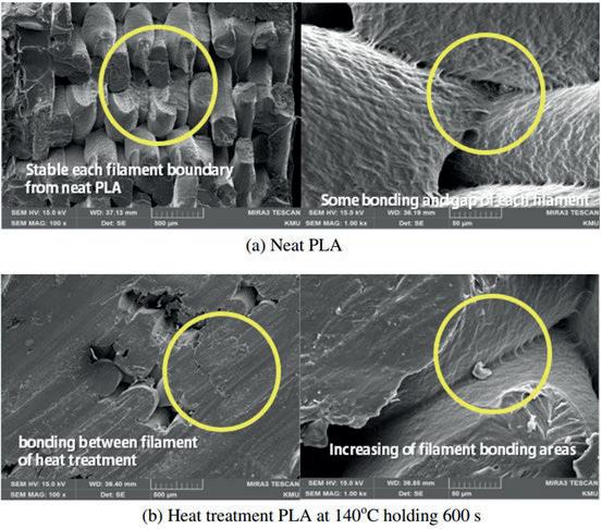
How do changes in layer height affect thermal annealing’s changes to the tensile strength of FFF printed parts?

Scientific Hypothesis

If layer height of ABS samples is decreased, then annealing will cause a larger percentage change in tensile strength.

Methodology

20 ABS samples were manufactured using the D638 type IV dog bone template (see Figure 2) at a layer height of 0.10mm, all samples were printed in the same orientation with the same file using the printing parameters in Table 1. 20 more samples each were then manufactured at layer heights of 0.15mm and 0.20mm, for a total of 60 samples manufactured. 5 samples of each layer height were then placed into a convection oven for 20 minutes at three temperatures being 120°C, 140°C and 160°C. Therefore 5 samples were collected for each temperature and layer height. The “Barker Bridge Buster 3000” (Figure 3) was then used to assess the force applied when each sample failed, and this data was recorded. A two-way ANOVA test was then used to analyse the means, variance and interaction between the two independent variables, comparing a calculated P-value against a predetermined ∝ (alpha) value of 0.05 to determine whether there were significant differences between the mean change in tensile strength.

Table 1: Printing parameters used

Results

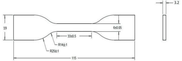
The relationship between layer height, temperature and tensile strength can be seen in Figure 4, where decreases in tensile strength across all layer heights are observed. The raw data collected for each layer height can be observed in Table 2, Table 3, Table 4. There is a general decrease in strength as the temperature increases for each of the layer heights tested, with a noticeable sharp drop in strength at the 160°C samples. The heat treated samples also presented with some warping in the corners but did present with noticeable shrinkage which could be a concern for manufacturers and future application.

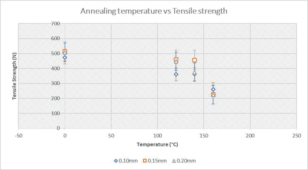
0.10mm Layer Height

The 0.10mm layer height group presented with lowest tensile strength when neat (neat meaning no post-processing treatments were performed), as expected. The percentage of strength compared to neat samples for each temperature were 83%, 86%, and 55% for the 120°C, 140°C and 160°C respectively (Table 5). The 120°C and 140°C data sets did include the outliers acknowledged below, so it is worth noting that the means used to calculate the percentage change are potentially not fully representative of the common data values seen for majority of samples. The variance for this 0.10mm group is relatively high compared to the 0.15mm and 0.20mm groups, indicating less consistency in its tensile strength as expected. The large standard deviation for 140°C and 120°C could be attributed to the outliers mentioned below, but since samples are being evaluated for both average strength and consistency, it was decided that these outliers would be kept and treated as normal.

Table 2: Raw tensile strength data for 0.10mm layer height samples.

0.15mm Layer Height

The 0.15mm neat samples were the strongest out of the three layer heights. Figure 4 shows 0.15mm samples also performing the best in the 120°C and 140°C temperatures. Both were 89% of the neat sample strength and the 160°C sample was 44% of the neat sample strength. The variance increases as temperature increased, and all variance values are relatively moderate, having no abnormally large variance values, compared to 0.10mm’s variances all exceeding 1200 (Table 2) or 0.20mm 140°C’s variance of 9555.31 (Table 4). This indicates a higher consistency for this layer height where all samples are being affected more similarly.

Table 3: Raw tensile strength data for 0.15mm layer height samples.

0.20mm Layer Height

The 0.20mm samples performed similar in strength for both neat and 120°C 0.15mm samples (Figure 4), where percentage strength of the neat samples were 88%, 74% and 44% for 120°C, 140°C and 160°C respectively. 44% for the 160°C sample was the same percentage strength of neat samples which was found in the 0.15mm, 160°C sample. The variance for the 0.20mm group at the lower temperatures (0°C and 120°C) are small and indicate less failure causing defects as expected (Table 4). However as temperature increases the variance also has large increases more similar to the lower layer height of 0.10mm’s 140°C and 160°C samples (Table 2).

Table 4: Raw tensile strength data for 0.20mm layer height samples.

Layer Height

0.2

1 Data values identified and acknowledged as statistical outliers, but since samples did not present noticeable physical defects and no machinery failed, they will be left in the data set since they contribute to the set’s variance and does provide insights into the interaction between annealing and layer heights.

Table 5: Percentage strength of specimens compared to the non-annealed control group.

Two Way ANOVA

As a method to analyse the data’s statistical significance, a two way ANOVA test was used with replication. The null hypotheses are:

1. There is no significant difference between the tensile strength means of the layer heights.

2. There is no significant difference between the tensile strength means of the temperatures.

3. There is no significant interaction between the layer height and temperature on the tensile strength.

The alternative hypotheses are:

1. There is a significant difference between the tensile strength means of the layer heights.

2. There is a significant difference between the tensile strength means of the temperatures.

3. There is a significant interaction between the layer height and temperature on the tensile strength.

The resultant values of the test are seen in Table 6, where the P-value for layer height was found to be 0.020321, and the P-value for temperature was found to be 1.10x10-16, and P-value for the interaction between variables was found to be 0.049468. Since 0.020321 is less than the ∝ (alpha) value of 0.05, we can reject the first null hypothesis. 1.10x10-16 and 0.049468 are also both less than 0.05 and therefore we can reject the second and third null hypotheses.

Therefore, the alternative hypotheses are all favoured, indicating that there is a significant difference between the means of the different layer height and temperature samples as expected. The third alternative hypothesis can also be favoured, which indicates a significant interaction between the layer height and annealing temperature, meaning layer height does change the effectiveness of the annealing process.

Table 6: Results of two way ANOVA test with replication. Columns refers to individual temperatures and rows are layer heights.

Discussion

This study aimed to evaluate the effects of differing layer heights and their influence on thermal annealing’s increases to strength. However, the data gathered suggested a decrease in tensile strength when annealed (Figure 4). Maximum tensile strength is known to occur at 105°C (Seok et al., 2023), but due to limitations in heating element and a desire to test a wider range of data values, this method started above this theoretical annealing temperature for maximum tensile strength. Therefore, it is possible that the annealing temperatures were too high. Additionally, many studies have found either minor increases in tensile strength for annealed ABS or even decreases (Hussam et al., 2025). The large decrease in tensile strength for 160°C is likely due to the temperature nearing the melting point, where the ABS becomes too viscous. The tensile strength means of 160°C samples being similar at 261N, 226N and 224N (Table 2, Table 3, Table 4) can also be explained by the ABS being

too viscous, as once it has become too viscous, the different layer heights are less distinguishable. Therefore we can assume that at higher temperatures nearing the melting point of ABS or a similar thermoplastic, the effect of layer height is minimised.

Given that there is a significant interaction between the layer height and temperature (Table 6) the effect of annealing will be determined through the percentage change compared to neat samples. Figure 5 indicates that samples printed at a layer height of 0.20mm were affected more heavily at the 140°C and 160°C temperatures. It also indicates 0.15mm samples to be less affected at the lower temperatures, but once it approaches the melting point, the tensile strength sees a sharp drop off. 0.10mm samples had moderate percentage change, noticeably having a lower change in 160°C tensile strength. These decreases and different changes in percentage are likely due to the existence of ‘voids’ formed between the layers (areas of little to no material) (Hussam et al., 2025). As

temperature increases, the cohesion between roads (layers) increases since the material is melting together, forming strong, solid blocks of material which are more difficult for cracks to propagate through. However, it can also be seen that as temperature increases, more voids form, particularly beyond the glass transition point (Hussam et al., 2025). This idea of voids being formed can explain the decrease in strength seen in the samples, particularly explaining the large decrease in tensile strength for 160°C samples, as this temperature is too high and allows the material to form more voids which cause major failures. The interaction between layer height and temperature, which was found to be statistically significant, on tensile strength can be explained as follows.

At higher layer heights where there is worse neck growth on neat samples, the lower temperature annealing process will improve the bonding which increases strength, combatting the creation of voids and their negative influence on tensile strength. As layer height decreases, there is better neck growth initially (Sood et al., 2010), and when annealed at lower temperatures, the neck growth has less improvement given the improved initial bonding. Therefore, the annealing process for these samples improves the strength less than the higher layers, meaning it combats the decreasing strength as a result of the creation of voids less, leading to a larger percentage decrease in tensile strength. At higher temperatures, the existing voids from the FDM manufacturing process are exacerbated, forming larger pockets which lead to a more violent decrease in percentage change of means (Hussam et al., 2025) Therefore, since larger layer heights generate parts

with more initial voids – due to their rougher print quality – at higher temperatures, the voids are exacerbated and cause the tensile strength to decrease. At lower layer heights, there is less room for voids to be initially generated, and therefore this issue is not magnified to the level it is in the higher layer height parts. These are indicated in Figure 5 where we can see at 160°C, 0.10mm has the smallest percentage change in means, decreasing by 45%, whereas the 0.15mm and 0.20mm samples both decreased in strength by 56%.

Limitations

This study had a couple key limitations. Mainly being the inability to find any increase in ABS tensile strength. This is a result of a combination of factors, mainly being the use of amorphous ABS, which is known to not have large increases in strength after annealing, along with a methodology which selected a wider range of temperature values at the expense of maximising the tensile strength.

Future Research

This project contributed to the current understanding of FFF ABS and its thermal annealing properties. Future research should focus on exploring different composites/materials such as PLA or nylon, which have different structures and respond differently to thermal annealing, could present different results or trends due to these unique properties and reactions to annealing. Additionally, varying temperature values around the glass transition point could offer new insights into the behaviour of these FFF layer by layer parts when thermally annealed.

Conclusion

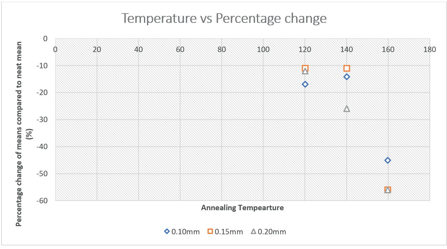
This research found a significant relationship between FFF layer height and thermal annealing’s effect on the tensile strength of ABS. The two way ANOVA test presented every variable to have a significant effect on tensile strength, indicating that there was some interaction between the layer height and temperature which changed the tensile strength at different percentages. This was explained through the two physical properties of neck growth (interlayer bonding) and voids. Where the lower layer height was theorized to have smaller improvements to neck growth, but less voids exacerbated at high temperatures. And conversely, the higher layer height would see larger improvements to neck growth, leading to less decrease in the lower temperatures, but more voids magnified due to the rougher construction as a result of the larger layers in the high temperature range.

Acknowledgements

I would like to thank Dr Matthew Hill for his guidance in idea generation and his consistent feedback and input to this study.

References

Blok, L. G., Woods, B. K. S., Yu, H., Longana, M. L., & Potter, K. P. (2017). 3D printed composites – benchmarking the state-of-the-art.

Butt, J., & Bhaskar, R. (2020). Investigating the Effects of Annealing on the Mechanical Properties of FFF-Printed Thermoplastics. Journal of Manufacturing and Materials Processing, 4(2), Article 2. https://doi.org/10.3390/jmmp4020038

Cano-Vicent, A., Tambuwala, M. M., Hassan, Sk. S., Barh, D., Aljabali, A. A. A., Birkett, M., Arjunan, A., & SerranoAroca, Á. (2021). Fused deposition modelling: Current status, methodology, applications and future prospects. Additive Manufacturing, 47, 102378. https://doi.org/10.1016/j.addma.2021.102378

Dawoud, M., Taha, I., & Ebeid, S. J. (2016). Mechanical behaviour of ABS: An experimental study using FDM and injection moulding techniques. Journal of Manufacturing Processes, 21, 39–45. https://doi.org/10.1016/j.jmapro.2015.11.002

Gao, X., Qi, S., Kuang, X., Su, Y., Li, J., & Wang, D. (2021). Fused filament fabrication of polymer materials: A review of interlayer bond. Additive Manufacturing, 37, 101658. https://doi.org/10.1016/j.addma.2020.101658

Goh, G. D., Yap, Y. L., Tan, H. J. K., Sing, S. L., Liang, G. G., & Yeong, W. Y. (2019). Process-Structure-Properties in Polymer Additive Manufacturing via Material Extrusion: A Review. https://doi.org/10.1080/10408436.2018.1549977

Hong, J.-H., Yu, T., Chen, Z., Park, S.-J., & Kim, Y.-H. (2019). Improvement of flexural strength and compressive strength by heat treatment of PLA filament for 3D-printing. Modern Physics Letters B. https://doi.org/10.1142/S0217984919400256

Hussam, H., Soliman, Me. S., Hassab-Allah, I. M., & Abdelrhman, Y. (2025). Effect of annealing on FDMmanufactured ABS parts. The International Journal of Advanced Manufacturing Technology, 138(5), 2233–2243. https://doi.org/10.1007/s00170-025-15455-5

Ligon, S. C., Liska, R., Stampfl, J., Gurr, M., & Mülhaupt, R. (2017). Polymers for 3D Printing and Customized Additive Manufacturing. Chemical Reviews, 117(15), 10212–10290. https://doi.org/10.1021/acs.chemrev.7b00074

Nagaraj, A., & Rajan, M. (2020). Chapter 19 - Future needs and trends: Influence of polymers on the environment. In M. A. A. AlMaadeed, D. Ponnamma, & M. A. Carignano (Eds.), Polymer Science and Innovative Applications (pp. 593–634). Elsevier. https://doi.org/10.1016/B978-0-12816808-0.00019-6

Seok, W., Jeon, E., & Kim, Y. (2023). Effects of Annealing for Strength Enhancement of FDM 3D-Printed ABS Reinforced with Recycled Carbon Fiber. Polymers, 15(14), Article 14. https://doi.org/10.3390/polym15143110

Sharma, M., Kala, P., & Sharma, V. (2019). (PDF) Optimization of process variables to improve the mechanical properties of FDM structures. ResearchGate. https://doi.org/10.1088/1742-6596/1240/1/012061

Singh, S., Singh, M., Prakash, C., Gupta, M. K., Mia, M., & Singh, R. (2019). Optimization and reliability analysis to improve surface quality and mechanical characteristics of heat-treated fused filament fabricated parts. https://doi.org/10.1007/s00170-018-03276-8

Sood, A. K., Ohdar, R. K., & Mahapatra, S. S. (2010). Parametric appraisal of mechanical property of fused deposition modelling processed parts. https://doi.org/10.1016/j.matdes.2009.06.016

Valvez, S., Silva, A. P., Reis, P. N. B., & Berto, F. (2022). Annealing effect on mechanical properties of 3D printed composites. Procedia Structural Integrity, 37, 738–745. https://doi.org/10.1016/j.prostr.2022.02.004

Wickramasinghe, S., Do, T., & Tran, P. (2020). FDMBased 3D Printing of Polymer and Associated Composite: A Review on Mechanical Properties, Defects and Treatments. Polymers, 12(7), Article 7. https://doi.org/10.3390/polym12071529

Investigation into the Efficiency of Novel Toroidal Propellers in Ground Effect

Angus Botham Barker College

Toroidal propellers are a novel propeller design which feature looped blades which lower noise and increase efficiency. Ground effects are changes in propeller behaviour as it approaches the ground, most notably an increase in efficiency and decrease in stability. The existing literature demonstrates that a traditional propeller (non-toroidal), increases in efficiency closer to the ground, and that away from the ground toroidal propellers are more efficient than traditional propellers. However, toroidal propellers have not been tested in ground effect conditions and there is a gap in research. In this report a range of traditional and toroidal propellers were tested at different heights and throttle settings to determine which propeller design’s efficiency is more impacted by ground proximity (ground effect). Toroidal propellers had an average peak efficiency gain 36% higher than traditional propellers, suggesting that wake pressure is the dominant factor in determining efficiency gains. Toroidal propellers’ higher efficiency increase solidifies their position in future UAV applications. The decrease in stability because of this needs to be addressed with suitable operating procedures.

Literature Review

A UAV (Unmanned Aerial Vehicle), commonly known as a drone, is a broad term referring to an uncrewed aircraft which operates remotely or autonomously (Fahlstrom et al., 2022). In recent years, the use of UAV rotorcraft has become increasingly widespread thanks to their uses in recreation, surveillance, photography and other applications (Muchiri & Kimathi, 2022). These drones use rotating propellers to generate lift and thrust similarly to a helicopter (Monteiro et al., 2022) Most drones utilise traditional fixed pitch propellers, which have been in use since the birth of powered flight (Rau, 2024)

Efficiency of Propellers

The propulsive efficiency of a propeller is a measure of how effectively a propeller converts input power to useful forward motion (Glover, 1986). A propeller with higher propulsive efficiency requires less input power to generate the same amount of kinetic energy.

This makes propellers with high propulsive efficiency a desirable due to their longer flight endurance, reduced power consumption and better handling (Benito & Alonso, 2018)

Propulsive efficiency is defined by the following equation (Lutz et al., 2009):

Where:

���������������� = Propulsive Efficiency

T = Thrust (N)

�������� = Velocity (ms-1)

P = Power Input (W)

The efficiency of a propeller is determined by many complex factors. Aerodynamic factors such as the propeller’s pitch (blade angle), aerofoil profile and number of blades affect how air behaves around the propeller (Wald, 2006). There are two types of drag which mostly impact how efficient a propeller is: parasitic and induced drag (Abdel-Motaleb et al., n.d.). Parasitic drag is caused by the propeller being in the way of air and having to force it out of the way and is proportional to velocity squared. Induced drag is a byproduct of lift, where air under the propeller has higher pressure than the air above it (Sadraey, 2009) The high-pressure air is sucked around the end of the blade, causing a spiralling airflow pattern called a wingtip vortex. This creates turbulence, which lowers propeller efficiency (Giuni, 2013). The complex airflow around a rotating propeller can be seen in Figure 2.

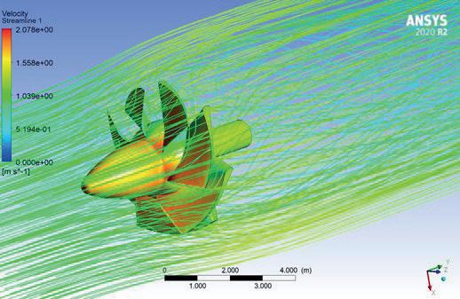
Propulsive efficiency, defined by Equation 1, can be understood as how well a propeller converts input energy into useful kinetic energy or forward motion, which is why there is a velocity term (Glover, 1986) This definition suits rockets and aircraft but is not useful to hovering drones where the propeller is not accelerating the craft. All hovering drones have zero propulsive efficiency since they are not gaining kinetic energy (Susi et al., 2025). A better measure of the efficiency of a hovering drone is the propeller efficiency, which will be expressed as �������� . This has been used in previous research and is the simplest measure of static efficiency.

Where:

�������� = Propeller Efficiency

T = Thrust (N)

P = Power (W)

It is not dependent on the velocity and kinetic energy of the drone, only the power input and thrust output of the propellers. In this report, propellers are tested in hover-like conditions, which is why the propeller efficiency will be used as it is the best measure of efficiency for the purposes of this report (Susi et al., 2025). From here on, the word ‘efficiency’ refers to the propeller efficiency, not the propulsive efficiency.

Ground Effect

Propellers experience ‘ground effect’ when within about 1D (1 propeller diameter) from the ground (Prouty, 1985, Tanabe et al., 2021). Ground effects are the changes in propeller behaviour when close to the ground, caused by the propeller’s wake airflow being blocked instead of flowing freely downwards, which increases wake pressure and dampens wingtip vortices (Betz, 1937). Due to the wake airflow being blocked by the ground, air under the propellers has higher pressure than the ambient air and thus pushes the drone upwards (Hadipour & Kamali, 2024). This leads

to a ‘free’ increase in thrust without drawing more power, increasing the efficiency. Below 0.5D, wake airflow is deflected by the ground and recirculates around the propeller, which can be seen in Figure 3 (Tanabe et al., 2021). This air interacts with the wingtip vortices as it passes them and dampens them. This decreases induced drag and hence increases the efficiency (Tanabe et al., 2021). Ground effect also increases instabilities and control issues since the higher pressure air between the propellers and the ground can oscillate and behave unpredictably as it escapes the region under the drone (Matus-Vargas et al., 2021). Figure 4 clearly shows how the power draw (and thus efficiency) with height for traditional propellers, and reduces below 1D (Schmaus et al., 2012, as cited in Tanabe et al., 2021)

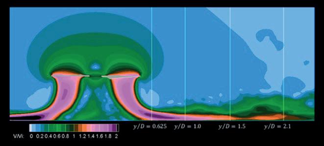
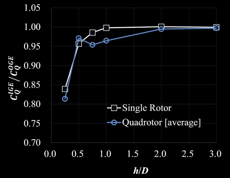
al., 2012, as cited in Tanabe et al., 2021)

Toroidal Propellers

Toroidal propellers are a novel propeller design with looped blades, designed by researchers at MIT (Sebastian & Strem, 2022). A diagram of toroidal propellers versus traditional propellers can be seen in Figure 5. They have been experimentally and computationally shown to generate less noise and achieve higher propulsive efficiency than traditional propellers (Ye et al., 2024). This has led to them slowly being adopted into UAV applications (Combey et al., 2024). These advantages are caused by the loop on the end of the blade, which acts similarly to the

winglet on an aircraft wing, blocking low and high pressure air from above and below the blade respectively from mixing and therefore reducing induced drag (Narayan & John, 2016). The thrust of toroidal propellers at high RPM ranges is more than twice as high as that of the equivalent traditional propeller (Ion & Simion, 2023). Toroidal propellers have a higher wake airflow velocity than traditional propellers, as seen in Figure 6. This is believed to be because of the looped blade having a nozzle effect, where the rear blade in the loop accelerates the air further before it leaves the propeller (Combey et al., 2024).

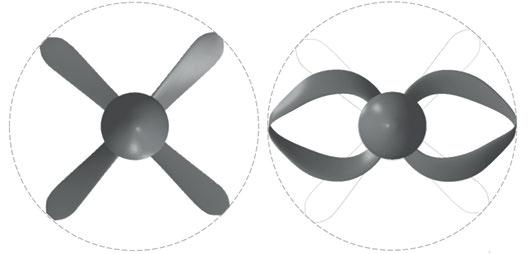
Toroidal Propellers in Ground Effect

It is unclear how toroidal propellers will behave in ground effect, since the factors that cause ground effect in traditional propellers are wingtip vortices and wake airflow, which both behave very differently on toroidal propellers. There is a gap in existing research as ground effect in toroidal propellers has not been simulated or experimentally investigated. There is no research about comparing ground effect between

different propeller designs in the same experimental setup, which is what this report aims to address.

Scientific Research Question

What effect does ground proximity have on the efficiency of toroidal propellers compared to traditional fixed pitch propellers?

Scientific Hypothesis

Toroidal propellers will experience less of an increase in efficiency than traditional propellers when close to the ground.

Methodology

Propellers

To test the propeller efficiency of different designs (hereafter referred to as “efficiency”), four different propeller designs were selected – two toroidal and two traditional. These were a two and four bladed traditional fixed pitch propeller, and a two and three looped toroidal propeller, which can be seen in Figure 8. The 2 blade and 2 loop propeller models were sourced online. They were copied and modified into the three loop and four bladed propellers, and then all propeller models were adjusted to the same specifications, as seen in Figure 7. The propeller designs were printed on a Bambu Labs P1S 3D printer in PLA. The exact print and design specifications, along with model sources, are available in Appendix B.

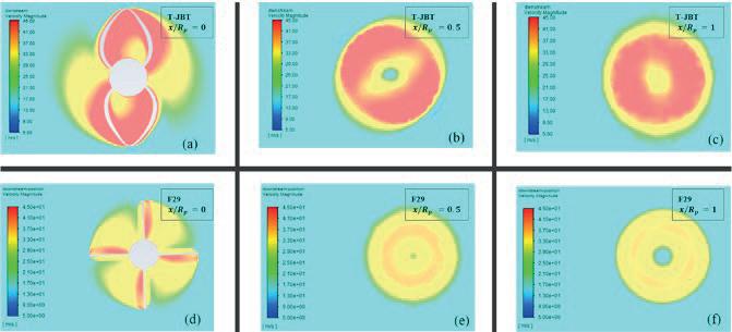
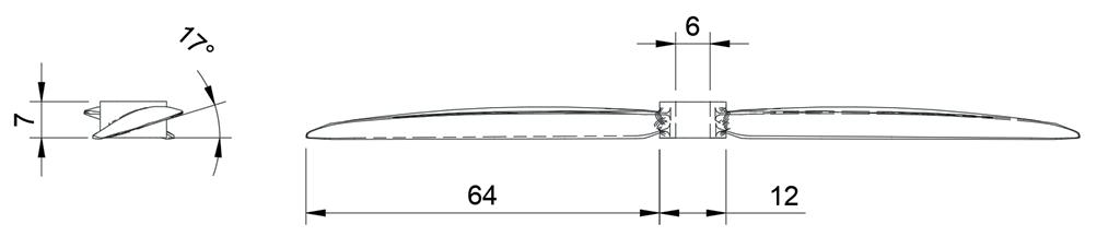
7: Propeller dimensions (consistent between all propeller designs). Dimensions are in millimetres.

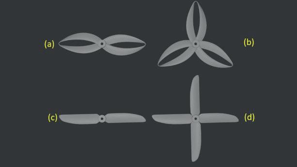
8: Render of propeller designs (a: 2 loop toroidal, b: 3 loop toroidal, c: 2 blade traditional, d: 4 blade traditional)

Apparatus

An apparatus was designed to test the propellers at different throttle settings and measure their thrust and power draw, as seen in Figure 9. It was able to do this at various heights above a flat stable surface so that the efficiency could be compared between heights. A 1000kV electric motor was attached to a 10kg load cell, which was held in a four-finger clamp on a retort stand. The load cell was wired to a HX711 load cell ADC (Analog to digital converter), and the electric motor was wired to an ESC (Electronic speed controller). The HX711 and ESC were zip tied to the other end of the clamp arm. The ESC’s power cable was connected to a Wattmeter and then into an 11.1V LiPo battery. The ESC’s signal wires and the wires coming out of the HX711 attached to an Arduino Uno development board. A 100k Ohm potentiometer was connected to the Arduino to allow user input, controlling the propeller throttle. The Arduino was plugged into a laptop running the Arduino IDE software to monitor thrust and throttle readings. A ruler was cable tied to the retort stand to measure the height of the propeller blades. A complete circuit diagram is available in Appendix C.

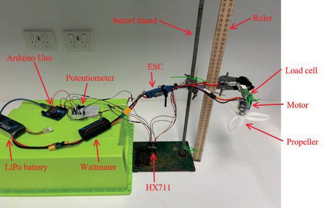
9: Side view of experimental setup. The arm of the retort stand could be raised or lowered to the desired height as measured by the wooden ruler. This allowed the propeller to be positioned at various distances from the ground to measure the relative ground effects.

Procedure

Four different propellers, two toroidal and two traditional, were operated at high angular velocity with equal throttle input and thrust and power draw were measured. The propellers were orientated horizontally above a flat, immovable surface such that airflow was pushed down towards the surface and thrust pushed upwards. Propellers were tested at distances between 300 to 20mm above the surface, at throttles of 40% and 80%. By measuring how the efficiency varied at different heights, the relative ground effects for different propeller designs could be compared.

Propellers were attached to the motor by unscrewing the collet adapter and placing a propeller on the thread. It was then put on the motor shaft and the hub tightened over the propeller. Each propeller was tested at 12 different heights: 300, 250, 200, 175, 150, 125, 100, 75, 50, 40, 30 and 20 mm. Each height was tested at 40% and 80% throttle. When a test was performed, the retort stand was first adjusted to the desired height. The Arduino was reset by uploading the code. When the laptop console started reading values, the battery was plugged into the wattmeter. The potentiometer was rotated clockwise until the throttle reading was at the desired value, and the power draw was recorded from the wattmeter. The potentiometer was set back to zero and the battery was unplugged. The average thrust value over a 5 second time period was recorded by the laptop automatically. The values of power draw and thrust for each test were recorded into a spreadsheet.

Data Analysis

The efficiency was calculated by dividing each thrust value by the corresponding power value. The efficiency values were then normalised by dividing each value by the value at 300mm. This was done to compare the relative change in efficiency with height

rather than directly comparing the efficiency between propellers. The efficiency gain was represented as a dimensionless decimal value. The data for each propeller was then graphed on a scatter plot, with the 40% and 80% throttle tests as different graphs. Each propeller design represents a data set on the graph.

Results

Figures 10 and 11 show the efficiency increase with ground proximity for each propeller.

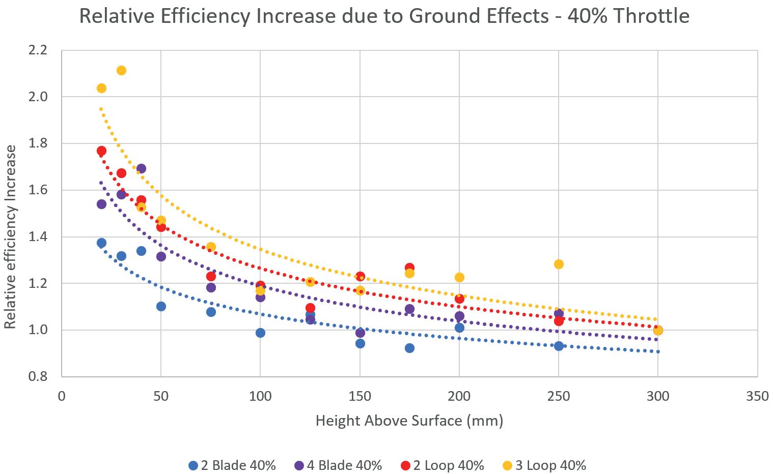
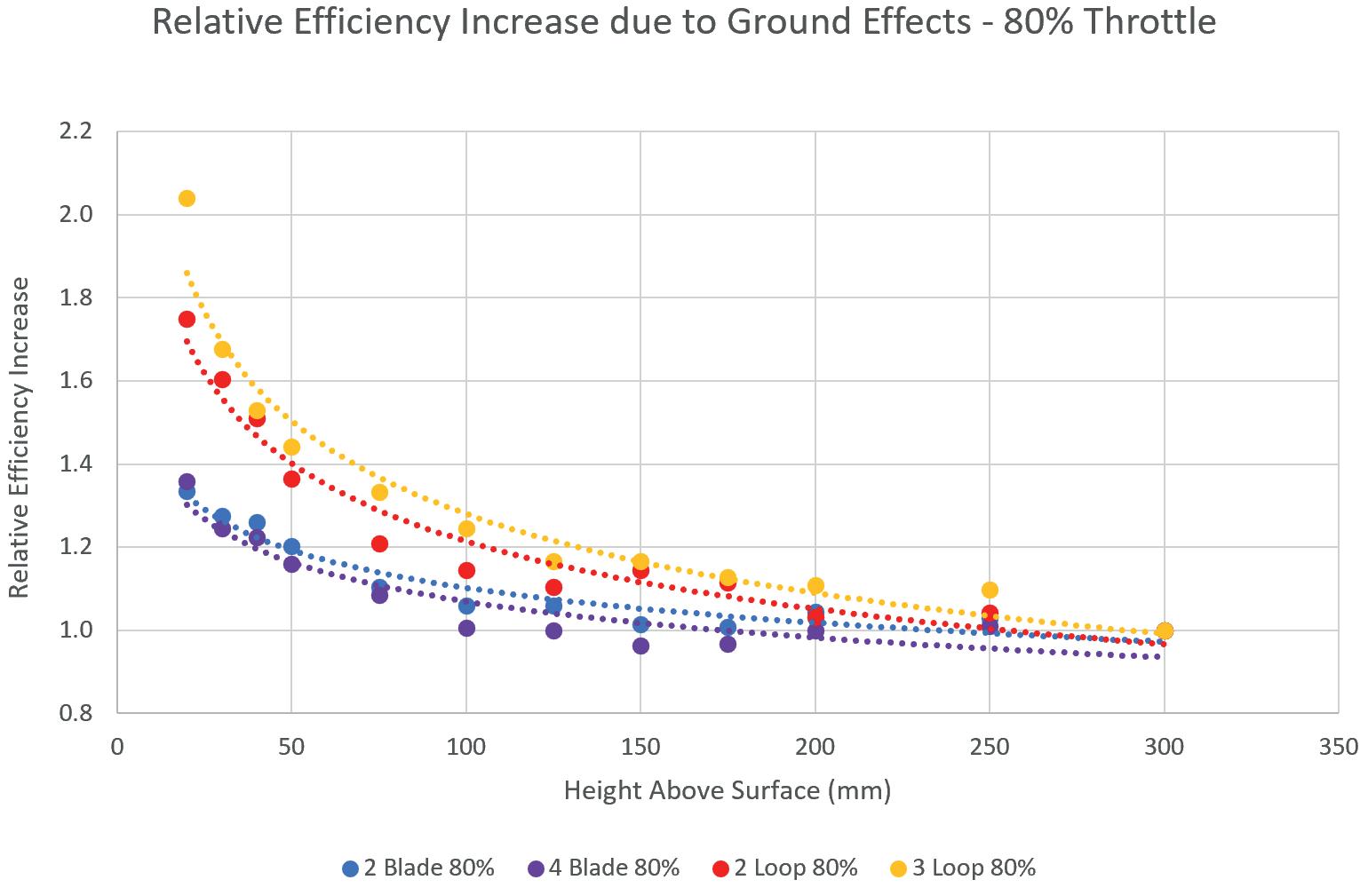
As expected, ground effects were experienced by all propellers on both throttle settings. By comparing the relative efficiency increase compared to the initial efficiency measurement at a height of 300 mm, the ground effects can be compared. Toroidal propellers (blue and purple data) had a much greater increase in efficiency as they were moved closer to the surface, which does not support the hypothesis.

Traditional Propellers

The two types of traditional propeller designs tested, 2-blade and 4-blade, both experienced an increase in propulsive efficiency when they approached the ground for both throttle settings. The relative efficiency increase fluctuated between 0.9 and 1.1 at heights 100 mm and higher. The 4-blade propeller’s efficiency increased up to a peak of 1.7 at 40 mm and dropped down to 1.5 at the lowest height for the 40% throttle tests but peaked at only 1.4 on the 80% tests. On both tests, the 2-blade propeller’s efficiency rose to 1.4, peaking at the lowest height. Efficiency increases were observed at heights below 100 mm, with major increases below 50 mm. Overall, the efficiency gain of the propellers was slightly greater for the 40% throttle tests.

Toroidal Propellers

Both toroidal propeller designs tested experienced an increase in propulsive efficiency as they approached the ground on both throttle settings. Efficiency fluctuated around 1 – 1.3 at heights above 100 mm for both 2 and 3-looped propellers on both throttle settings. The 2-loop propeller’s efficiency peaked at 1.8 at the lowest height for both throttle settings. The 3-loop propeller’s efficiency peaked at 2.0 for the 80% tests and 2.1 for the 40% tests. Both toroidal propeller designs behaved similarly except for the 3-loop propeller’s much higher peak efficiency gain. This suggests that the number of loops does impact ground effects.

Discussion

Comparison of Results

Overall, the toroidal propellers experienced a greater increase in efficiency as the propeller was positioned closer to the ground than the traditional propellers. This does not support the original hypothesis which suggested positive ground effects would be more pronounced for the traditional propellers. The efficiency increase for the 40% throttle tests was 31.2% higher on average for the toroidal propellers than the traditional ones. Similarly, the efficiency increase of toroidal propellers at 80% throttle was 40.7% higher than the traditional propellers. As can be seen in Figures 10 and 11, The toroidal propellers started experiencing ground effects slightly higher

than the traditional propellers did for both throttle settings. All propellers efficiency had much less random error on the 80% throttle tests, producing a much smoother graph.

Explanation of Results

The results do not support the original hypothesis and show that toroidal propellers are impacted more by ground effect than traditional propellers. The prediction was due to an overestimation of the effect of wingtip vortices on efficiency versus wake pressure. As the results indicate the opposite (the efficiency of toroidal propellers was experimentally shown to increase up to 50% more than on traditional propellers) an alternative explanation needs to be explored.

A propeller’s mass flow rate (the rate at which the substance, in this case air, moves through the propeller) is given by the equation (Ewart et al., 2006):

Where:

�������� = Mass Flow Rate (kgs-1)

�������� = Air density (kgm-3)

���������������� = Disc Area (m2)

���������������� = Wake Airflow Velocity (ms-1)

According to this equation, an increase in wake airflow velocity leads to an increase in mass flow rate. The mass flow rate is linked to pressure by the ideal gas law (Garret, 2020):

(2)

Where:

�������� = Absolute Pressure (Pa)

�������� = Volume (kgm-3)

�������� = Amount of Substance (mol)

�������� = Universal Gas Constant

�������� = Temperature (K)

When there is a surface close to the tailing end of the propeller, a higher mass flow rate leads to ��������, the amount of air under the propeller, increasing. The ideal gas law says that a higher quantity of air under the propeller leads to higher pressure.

Pressure is defined by the formula:

(3)

Where:

�������� = Absolute Pressure (Pa)

�������� = Force (N)

�������� = Area (m2)

This means that a higher pressure under the drone increases the force pushing outwards. Therefore, the drone and propellers are pushed upwards by the highpressure air, effectively giving it a boost in thrust (Betz, 1937). This means that toroidal propellers increase the thrust of a drone hovering close to the ground and thus increase its efficiency due to their higher wake airflow velocity compared to traditional propellers (Combey et al., 2024). Figure 12 shows the wake pressure under the drone at different heights, clearly revealing that the obstruction from the ground causes an increase in pressure and thus thrust and efficiency (Tanabe et al., 2021)

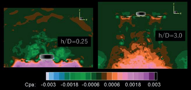
12: Simulated pressure distribution around a hovering quadcopter drone using traditional propellers (Source: Tanabe et al., 2021)

Another factor that causes ground effects is the dampening of wingtip vortices at low altitude, which decreases induced drag and increases efficiency. This effect would be much more pronounced on traditional propellers, since they have much larger wingtip vortices, and thus more efficiency to gain by dampening them (Giuni, 2013). It’s likely that traditional propellers’ get most of their efficiency increase from their wingtip vortices being dampened (Light, 1993). Traditional propellers wouldn’t gain as much efficiency from the wake airflow as toroidal propellers, since it is slower and hence the wake pressure is lower.

Toroidal propellers and traditional propellers get their efficiency increases mostly from different phenomena. Based on the results, the increased wake pressure from higher wake airflow velocity is the dominant effect on the efficiency increase of a propeller, not the dampening of wingtip vortices as was suggested in the literature. This is consistent with Figure 12, which does not show a noticeable decrease in wingtip vortex size with ground proximity like much of the existing research has claimed (wingtip vortices are the green circles next to the propellers). This explains how the toroidal propellers experienced a much higher efficiency increase than traditional propellers.

Implications of Results

Toroidal propellers experience a greater efficiency increase than traditional propellers when close to the ground. This means that drones equipped with toroidal propellers will be more efficient when flying close to the ground compared to traditional propellers. Increased efficiency leads to longer flight endurance and less energy use while operating. This also means that drones using toroidal propellers can be more unstable since the higher-pressure air underneath can oscillate and behave unpredictably as the air tries to escape the high-pressure region. The limited accuracy and speed of an autonomous drone’s instruments can further exacerbate this effect. This is because the delay between a measurement and the drone adjusting its flight accordingly is noticeable and can cause overcorrections and instability. UAVs can usually land while keeping ground effect instability under control, however sustained hovering can lead to more control issues (Matus-Vargas et al., 2021). Relevant operating procedures should be developed accordingly to minimise ground effect instabilities while operating at low altitudes.

Limitations and Future Research

The experimental setup was not perfect and had some design flaws which would have slightly impacted airflow. The ruler was quite close to the propeller and could have impacted airflow behaviour. Since the dominant factor in determining ground effects seemed to be wake pressure, the ruler probably didn’t make a huge difference since it wasn’t disrupting air under the propellers. The ruler could have impacted flow recirculation, but this didn’t seem to be a major factor so overall the ruler probably did not make much difference to the results.

To verify the assertion that wake airflow velocity is a more dominant factor in ground effect than dampening of wing tip vortices, the wake airflow velocity should be measured. This could be done with an anemometer under propellers, and wake pressure could be calculated to approximate the force pushing up on the propeller from ground effects. Through simulations the level of dampening of wing tip vortices could be ascertained to help confirm the reason as to why traditional propellers were less affected by ground proximity. An important factor in this would be to control for exact RPM ranges since the propellers had different masses so they would have been at different speeds.

Wider applicability of the results could be achieved through generalising the initial conditions. This would include investigating cases where a propeller is

hovering above a non-horizontal surface or testing different aerofoil designs.

Conclusion

Experimental analysis has revealed that toroidal propellers experience a greater efficiency increase in ground effect than traditional propellers do. At the lowest heights, toroidal propellers had an average peak efficiency gain 36% higher than traditional propellers, at up to 2.1 times higher than the original value. This result did not support the original hypothesis and challenges the accepted notion that the dampening of wingtip vortices is the main cause of ground effect. Based on evidence from this report and some existing literature, wake pressure is the main cause of ground effect in hovering drones. This explains why toroidal propellers experienced higher efficiency gains, as they have higher wake airflow velocity and thus higher wake pressure, which increases thrust.

Acknowledgements

I would like to thank Dr Matthew Hill for his supervision and guidance throughout my project, without whom this would not have been possible.

I wish to thank Mr Colin Jaques and Mr Stephen Liseo for their valuable contributions to my experimental design and setup. Without their expertise with propellers and circuitry, my experiment would not have been possible.

References

Abdel-Motaleb, S. A., Taylor, J. D., Hunsaker, D. F., & Coopmans, C. (n.d.). Comparison of Induced and Parasitic Drag on Wings with Minimum Induced Drag. In AIAA Scitech 2019 Forum. American Institute of Aeronautics and Astronautics. https://doi.org/10.2514/6.2019-2120

Benito, A., & Alonso, G. (2018). Energy Efficiency in Air Transportation. Butterworth-Heinemann.

Betz, A. (1937, August 1). The ground effect on lifting propellers. https://ntrs.nasa.gov/citations/19930094580

CFDSource. (2023, December 12). CFD Analysis of Propellers. CFDSource. https://www.cfdsource.com/ShowBlog/cfd-analysis-ofpropellers/

Combey, K., Elsayed, O., Qaissi, K., Faqir, M., & Chouiyakh, H. (2024). Aerodynamic Investigation of Novel Toroidal Joined Blade Tips Propeller

Ewart, T., Perrier, P., Graur, I., & Gilbert Méolans, J. (2006). Mass flow rate measurements in gas micro flows. Experiments in Fluids, 41(3), 487–498. https://doi.org/10.1007/s00348-006-0176-z

Fahlstrom, P. G., Gleason, T. J., & Sadraey, M. H. (2022). Introduction to UAV Systems. John Wiley & Sons.

Garret, S. (2020). Understanding Acousics (2nd ed.). ASA Press. https://link.springer.com/chapter/10.1007/978-3030-44787-8_7

Giuni, M. (2013). Formation and early development of wingtip vortices

Glover, E. J. (1986). Propulsive devices for improved propulsive efficiency. Transactions, 99(1). https://library.imarest.org/record/2292/files/2319.pdf

Hadipour, M., & Kamali, R. (2024). Experimental and Numerical Investigation of Propeller Propulsion System Behavior Considering the Ground Effect. Unmanned Systems, 1–12. https://doi.org/10.1142/S2301385025500712

Ion, G., & Simion, I. (2023). Performance of 3D printed conventional and toroidal propeller for small multirotor drones. Journal of Industrial Design and Engineering Graphics, 18(1), Article 1.

Light, J. S. (1993, April 1). Tip Vortex Geometry of a Hovering Helicopter Rotor in Ground Effe...: Ingenta Connect

https://www.ingentaconnect.com/content/ahs/jahs/1993/00 000038/00000002/art00004;jsessionid=24erdfge1q8n6.xic-live-02

Lutz, T., Funk, P., Jakobi, A., & Wagner, S. (2009). Calculation of the Propulsive Efficiency for Airships with Stern Thruster. AIAA Lighter-Than-Air Technical Committee Convention and Exhibition, Akron, Ohio, USA, 14th Edition.

Matus-Vargas, A., Rodriguez-Gomez, G., & MartinezCarranza, J. (2021). Ground effect on rotorcraft unmanned aerial vehicles: A review. Intelligent Service Robotics, 14(1), 99–118. https://doi.org/10.1007/s11370-020-003445

Monteiro, M., Stari, C., Cabeza, C., & Martí, A. C. (2022). Simple physics behind the flight of a drone. Physics Education, 57(2), 025029. https://doi.org/10.1088/13616552/ac484a

Muchiri, G. N., & Kimathi, S. (2022). A Review of Applications and Potential Applications of UAV. Proceedings of the Sustainable Research and Innovation Conference, 280–283.

Narayan, G., & John, B. (2016). Effect of winglets induced tip vortex structure on the performance of subsonic wings. Aerospace Science and Technology, 58, 328–340. https://doi.org/10.1016/j.ast.2016.08.031

Prouty, R. (1985). Ground effect and the helicopter A summary. In Aircraft Design Systems and Operations Meeting. American Institute of Aeronautics and Astronautics. https://doi.org/10.2514/6.1985-4034

Rau, V. (2024). A Computational Analysis of Toroid Propellers. AIAA Student Journal. American Institute of Aeronautics and Astronautics

Sadraey, M. (2009). Drag Force and Drag Coefficient. Aircraft Performance Analysis

Schmaus, J., Berry, B., Gross, W., & Koliais, P. (2012). Experimental Study of Rotor Performance in Deep Ground Effect with Application to a Human-Powered Helicopter

Sebastian, T., & Strem, C. (2022). Innovation Highlight: Toroidal Propeller. MIT. https://www.ll.mit.edu/sites/default/files/other/doc/2023-

02/TVO_Technology_Highlight_41_Toroidal_Propeller.pd f

Susi, J., Unt, K.-E., & Heering, S. (2025). The Efficiency of Drone Propellers A Relevant Step Towards Sustainability. Engineering Proceedings, 90(1), Article 1. https://doi.org/10.3390/engproc2025090089

Tanabe, Y., Sugawara, H., Sunada, S., Yonezawa, K., & Tokutake, H. (2021). Quadrotor Drone Hovering in Ground Effect. Journal of Robotics and Mechatronics, 33(2), 339–347. https://doi.org/10.20965/jrm.2021.p0339

Appendix A: Propeller Relative Efficiency Gain

Wald, Q. R. (2006). The aerodynamics of propellers. Progress in Aerospace Sciences, 42(2), 85–128. https://doi.org/10.1016/j.paerosci.2006.04.001

Ye, L., Wang, C., Guo, C., & Chin, J. (2024). Mathematical expression method for geometric shape of toroidal propeller. https://www.shipresearch.com/en/article/doi/10.19693/j.issn.16733185.03419?viewType=HTML

Appendix B: Propeller Specifications

Propeller Sources

Traditional propeller model: https://grabcad.com/library/improved-gemfan-5040-propeller-1

Toroidal propeller model: https://grabcad.com/library/toroidal-5040-propeller-1

Propeller Specifications

These models were adapted in Blender and the number of blades changed, so the aerodynamic characteristics of the individual blades were maintained between the two designs of each propeller. This means that the 2 and 4-blade traditional propeller, for example, are derived from the same model off the internet.

Print Specifications

Slicing software: Bambu Studio – Bambu Lab

Printer: Bambu Lab P1S

Plate: Textured PEI plate

Nozzle: 0.4 mm stainless steel

Print material: White PLA

System presets: Generic PLA, 0.16 mm High Quality

@BBL X1C

Layer height: 0.16 mm

Initial layer height: 0.2 mm

Seam position: Aligned

Wall loops: 3

Top surface pattern: Monotonic line

Top shell layers: 5

Top shell thickness: 1

Bottom surface pattern: Monotonic

Bottom shell layers: 4

Bottom shell thickness: 0

Internal solid infill pattern: Rectilinear

Sparse infill density: 45%

Sparse infill pattern: Gyroid

Support type: Tree (auto)

Threshold angle: 25°

Appendix C: Experiment Circuit Diagram

The Aerodynamic Performance of Two Hot Stages for Starship Super Heavy

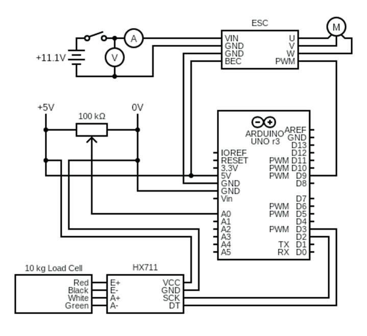
William Paterson Barker College

As SpaceX works to develop a fully reusable launch vehicle, hot staging has been adopted to increase payload capacity. Hot staging is when a multistage rocket ignites its upper stage while the lower stage is still firing, and requires a special vented interstage to vent exhaust. SpaceX has iterated through two designs; the Version 1 retrofitted adaptor and the Version 2 integrated hot stage. A CFD analysis was performed on both using SOLIDWORKS 2023 Flow Simulation to determine drag during subsonic flight at 70 m/s. It was found that the Version 1 design produced 11,065 N, and the Version 2 design produced 14,898 N, significantly worse than V1.

Literature Review

Starship Super Heavy

Starship Super Heavy is an in-development fully reusable super heavy lift launch vehicle built and operated by SpaceX (SpaceX, n.d.). It is intended to become the largest launch vehicle ever, both in terms of payload capacity and size. The entire vehicle, usually called Starship, consists of two stages; the upper stage is officially named Starship, but is generally referred to simply as the ship, while the booster is named Super Heavy, but booster is usually used instead (SpaceX [@SpaceX], 2025a). In this report, Starship will be used for Starship Super Heavy, ship will be used for Starship (V2 unless specified otherwise), and booster will be used for Super Heavy.

Starship’s design is unique in that it is slated to become the first fully reusable orbital rocket. Booster reuse has been achieved before (Falcon 9/Heavy), and the shuttle’s orbiters were each flown at least 10 times, but complete reuse has never been attempted. Super Heavy has been landed 3 times and reflown once, while the ship has made three successful soft touchdowns in the ocean and is likely to be caught by the ‘chopsticks’ in 2026.

Both the ship and booster are made from 4 mm 304L stainless steel (a type of steel mix with low carbon), chosen due to high heat tolerance, low cost, ease of manufacture, and acceptable weight. Lower mass alternatives such as carbon fibre and aluminium were considered during early revisions but dropped due to cost and manufacturability concerns

The ship

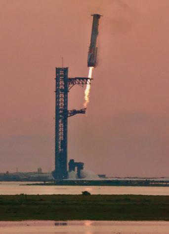
The flight version of the ship has flown in two configurations – Version 1 and Version 2 (Block 1 and Block 2 are terms also used). Significant changes were made between the two variants, most importantly for this report to the forward flaps. Other changes were internal, or negligible for the purposes of this report (slightly redesigned heat shield edge, lift point changes, changed internal reinforcements, etc). The forward flaps were moved from 180° to ~140° apart, shifted higher and towards the leeward side (Figure 3). They were shrunk, with a more swept design. The fuselage was extended by one barrel section (1.8 m), and the dry mass reduced by ~15 t (Jax, 2024a)

Figure 3: Starship V1 and V2 overlaid, showing the diametrically opposed V1 forward flaps compared to the more offset V2 flaps (Source: ChameleonCircuit (@ChameleonCir) / X, 2024)

The ship is 52.1 m tall, with a 9m diameter. Its dry mass is 85 t with an additional 1500 t of propellant (SpaceX, n.d.). It is powered by 3 gimballed Raptor 2 (Raptor) engines and 3 fixed Raptor 2 Vacuum (RVac) engines, which are kept within the engine ‘skirt’. The unpressurised space in the skirt is capped with a false ceiling which covers the aft dome of the propellant tanks, as well as the engine plumbing. The windward side is protected by a tiled, silica-based heat shield made up of ~18,000 hexagonal tiles. Re-entry is performed dissimilarly to the Space Shuttle, where instead of gliding it adopts a skydiver-like position (SpaceX [@SpaceX], 2025a). This entry is controlled by four hinged flaps – two forward flaps and two aft flaps – that independently rotate to provide pitch, roll, and yaw control. It transitions from falling horizontally to a vertical landing with a rapid pitch up controlled by both the flaps and the engines gimballing. Landing will be performed similarly to the booster, using the ‘chopsticks’ to catch the ship by its lift points. This controlled entry and landing is necessary for reusability (Elon Musk [@elonmusk], 2025).

The booster

The Super Heavy booster is of more conventional design than the ship and resembles the Falcon 9 booster somewhat. It is the same 9 m diameter of the ship, 71 m tall (including the hot stage), and has a dry mass of ~275 t (SpaceX, n.d.). The engine bay in the aft section features 33 Raptor 2 sea level engines – 20 fixed outer engines and 13 centre engines with gimballing and relight ability – which combined produce ~75.5 MN of thrust. The main fuselage is made of cylindrical barrel sections welded together, all the way up to the forward section. This is similar in construction to the rest of the booster but features four steel grid fins for aerodynamic control on entry. Mounted to the forward section is the vented interstage. The Version 2 booster will have one less grid fin than the Version 1 (Ringwatchers, 2024)

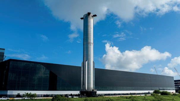
To simplify the simulation, the grid fins have been omitted. Due to their position aft of the interstage they interact minimally with the hot stage (Dominique Charbonnier et al., 2022; Marwege et al., 2022), and their complex shape majorly increases all computation times.

The hot stage

The hot stage, or vented interstage, is the part of the vehicle between the ship and booster which allows exhaust gases to escape during staging. On Version 1 boosters, this interstage is a retrofit which attaches to the clamps originally designed to hold the ship during ascent. It’s essentially a barrel section with many slot cutouts to maximise vent area. To protect the forward section of the booster (which houses flight controllers, grid fin motors, and the forward propellant tank dome) from hot exhaust, a blast shield redirects the exhaust outwards (Golden, 2024a, 2024b; Jax, 2023).

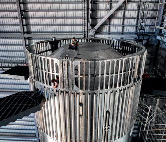
(Source:

2023). Note that it is not welded on, but a removeable adapter.

Version 2 boosters will feature an integrated interstage with a completely different design to the original. It is instead made of steel rods arranged in a truss structure mounted to the tank walls and a top ring (Figure 6). The blast shield is replaced with a thicker, reinforced forward dome (SpaceX, n.d.; SpaceX [@SpaceX], 2025b)

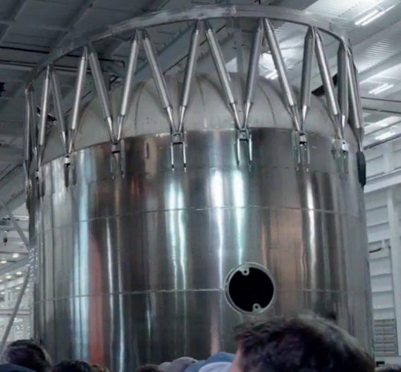
Figure 6: The Version 2 hot stage (Source: SpaceX [@SpaceX], 2025c). It is integrated with the structure of the booster, and has far more vented area.

Hot staging

Hot staging is the process of igniting an upper stage while the lower stage is still attached and firing. By avoiding time spent in free fall between stage separation and upper engine start, performance is majorly increased – by 10% in the case of Starship (Jeff Foust [@jeff_foust], 2023). While this payload advantage is significant, it is unclear how the increased drag from the hot stage will affect Starship prior to hot staging.

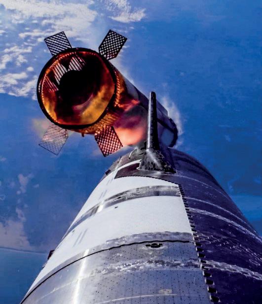
7: The booster detaching from the ship during hot

(Source: Elon Musk [@elonmusk], 2024). The photo was taken from a camera on the forward flap, looking aft.

Flight 9

Starship Flight 9 was launched on the 27th of May 2025. It is the most recent flight as of June 2025 and is what this report will be based off. It launched Starship Ship 35, a V2 ship, and the reused Booster B14-2, a V1 booster (where the -2 indicates a second flight). Its hot stage was V1. Several online sources,

such as Wikipedia, state incorrectly that B14 was a Version 2 booster which is incorrect; it is of the same basic design as all previous boosters since B7. As the V2 ships were ready before the V2 boosters, they are flown on an older booster generation.

Scientific Research Question

How does drag in subsonic flight differ between the V1 and V2 hot stage designs for Starship Super Heavy?

Scientific Hypothesis

The V2 hot stage will create less drag than the V1 hot stage.

Methodology

Four parts were designed in the CAD program SOLIDWORKS 2023 Education Edition as SLDPRT files. These parts were:

1. A Version 2 ship

2. A Version 1 booster without a hot stage

3. A Version 1 hot stage

4. A Version 2 hot stage

All models were simplified by omitting stringers, heat shield tiles, chines, grid fins, and outer raceways (Грибанова, 2025). No internal sections were included, as they were not used for the simulations.

The ship was designed using publicly available data for height and diameter (52 m tall, 9 m diameter). The nosecone section was modelled with reference to photographs of the nosecone prior to installation. The flaps were designed similarly, using the known ship diameter to determine dimensions based off photographs. The false ceiling was modelled as a flat panel 2.95 m from the base of the ship, determined from weld marks visible on the exterior of the ship.

The booster was designed as a simple closed tube with dimensions acquired from SpaceX’s website. The aft

section was not modelled, as it was not included in the computational domain.

The V1 hot stage was modelled with reference to photographs in a similar way. 45 cutouts with dimensions found from photographs were evenly spaced around the wall of the hot stage.

The V2 hot stage was modelled with reference to photographs, with 44 bars evenly spaced in a truss structure around the perimeter of the hot stage.

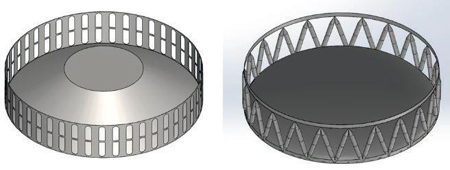
respectively, viewed from above.

Two assemblies were created: one with a ship, V1 hot stage, and booster, and the other the same with a V2 hot stage. A flow simulation was set up with the input data shown in Table 1 and the computational domain shown in Table 2 (for both assemblies). The global mesh was set to an accuracy level of 6, with the type ‘automatic’. Both simulations were then run and allowed to converge automatically. To produce data from these simulations, the SOLIDWORKS Surface Parameters tool was used. All surfaces were selected, and the parameters Normal Force, Friction Force, and Force were chosen, and exported into an Excel file.

Pressure, temperature, and velocity data was obtained from the broadcast of Starship Flight Test 9 at T+20 s. This was chosen due to Starship’s angle returning to near-vertical (on liftoff there is a slight tilt for a pad avoidance manoeuvre), and altitude being sufficient to exclude any ground effect or pressure difference caused by the launch pad itself.

Table 1: Input data used in the flow simulation.

Parameter Value

Analysis type External

Geometry recognition CAD Boolean

Exclude cavities without condition True

Exclude internal space True

Fluid Air

Flow type Laminar only

High Mach number flow False

Humidity False

Default wall thermal condition Adiabatic wall

Roughness 0.5 µm

Pressure 1.0142 bar

Temperature 28°C

Velocity parameters Velocity

Defined by 3D Vector

Velocity in X/Y direction 0 m/s

Velocity in Z direction -70 m/s

Results

All analysis were performed with the co-ordinate system: +Z as up when the vehicle is vertical for launch, +Y as the side the forward flaps are offset towards, and +X as the port side of the vehicle. In sideby-side comparisons, the V1 hot stage will be placed at the top or on the left of the figure.

Visual analysis

The two results were analysed visually using built-in SOLIDWORKS Flow Simulation tools. All analysis in this section is qualitative and non-rigorous. Figure 9 provides a visual overview of the two hot stages side by side. It can be seen that both of the simulations produce visually similar plots outside of the hot stage, with significant differences only occurring within the hot stage itself. There is a high-pressure zone appearing on the nose of the ship, giving way to a lowpressure zone lower on the nosecone. Streamlines smoothly flow around the nosecone and down the body of the vehicle, nearly parallel to the long axis of the rocket.

The close-up on the hot stages in Figure 10 gives more insight. The +Y axis is to the right of both images, and the difference in vortices between the -Y and +Y sides is similar across both designs. The +Y vortex is lower and closer to the blast shield and appears noticeably stronger than the -Y vortex in the V2 design with a lower pressure. The V2 vortices are both closer to the centre of the hot stage. In both designs around where the blast shield connects to the barrel sections, a highpressure zone is visible, which is a result of airflow being compressed by an obstacle (the struts). The high-pressure zone appears noticeably larger and higher pressure in the V2 design, but this is misleading as this high-pressure zone is present along the full circumference of the ring on the V1 hot stage, but only where the struts meet the barrel on the V2 hot stage; Figure 11 points this out. It can be seen that the majority of the hot stage does not cause this impediment to the flow and will not cause this highpressure zone, as confirmed by Figure 12.

Table 3: V1 hot stage results.

Table 4: Table 5: V2 hot stage results.

Quantitative analysis

The V1 hot stage produced substantially less drag than the V2 hot stage, by almost 4 kN, as can be seen in tables Table 3 and Table 4. While Z force was the major factor in the net force, as expected, Y force changed by a moderate ~570 N between the two hot stages. Both designs experienced a large +Y normal force with almost no friction force in that direction, which is likely lift produced by the flaps.

Discussion

It was found that the V1 hot stage design is better aerodynamically in the subsonic region of flight, which contradicts the hypothesis. The exact reason for this is difficult to determine using the tools available for SOLIDWORKS Flow Simulation, but there are some possibilities.

The larger clearance between the blast shield and the false ceiling (Figure 10) created more space for larger vortices to form without obstruction. Vortices form low-pressure zones which majorly increase drag in other flying vehicles such as aeroplanes (Spalart, 1998), and likely has a similar effect on Starship.

Another option, which is likely, is that the V2 hot stage is optimised for supersonic flight as opposed to subsonic. Starship spends almost all of its flight supersonic and drag is majorly increased during this region of flight, so it’s logical to optimise design of hot stages for supersonic flight. The aerodynamics of supersonic and subsonic flight differ significantly (“Research in the Region between Subsonic and Supersonic Speeds,” 1947) and an optimal design for subsonic flight in aeroplanes almost never corresponds to optimal supersonic design. The aerodynamics of supersonic flight are extremely complex (“Research in the Region between Subsonic and Supersonic Speeds,” 1947), and out of scope for this report. Future research building on the hypothesis of optimisation for supersonic flight is warranted.

Another possibility is that the reduction in mass was an acceptable trade-off for the increased drag. The V1 hot stage is heavy (Gee et al., 2024; Golden, 2024a, 2024b), and increased mass negatively affects a launch vehicle for the entirety of ascent, while aerodynamic effects become less impactful as the atmosphere thins (Dukeman, 2002). Trade-offs are most of the challenge of rocketry, and without detailed information only obtainable from internal SpaceX data, finding whether this is the case is difficult.

There were numerous limitations and improvements possible with the simulation. The most significant was the omission of engines on Starship. Unfortunately, changes in Raptor are constant and the move to Raptor 3, which doesn’t use engine shielding, was announced too late for the simulation to be rerun and reanalysed with the new variant. It was decided to instead not include engines, as their complex shape and relatively minimal impact on airflow increased computation time significantly without majorly impacting results. A custom mesh would have also been optimal for accuracy, but for time reasons the mesh was automatically generated (Figure 13). While suitable, the mesh’s accuracy and precision around critical points was lower than ideal, while simple surfaces like tank walls were too detailed.

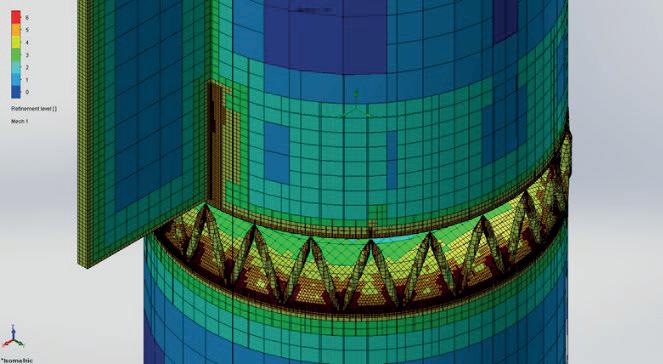
A more advanced and comprehensive simulation tool would have further increased accuracy. SOLIDWORKS Flow Simulation is best used for smaller assemblies with simple, low complexity

geometry (Matsson, 2023); aerospace applications generally use CATIA, another product by Dassault Systèmes (Dassault Systèmes, 2022). CATIA is complex, computationally intensive and far more difficult to access through school subscriptions than SOLIDWORKS but would have produced better results.

The reason for this result is likely to do with the amount of open space in the hot stage. A flat, unbroken cylindrical section will produce less drag than an equivalent section with cutouts, and the more cutout there is, the worse this gets. This can be thought of similarly to driving with car windows down – the smooth shape is broken up by the window holes, and aerodynamics are negatively affected (Viviani et al., 2016). The problem with hot staging is the requirement of as much open space as possible to vent exhaust gases, to avoid pressure buildup and damage to the upper stage or booster. However, if the claimed 10% payload boost is accurate, the efficiency gain from hot staging more than makes up for this issue.

Conclusion

Through two simulations using SOLIDWORKS Flow Simulation, the aerodynamics of Starship’s V1 and V2 hot stages were compared. The V1 hot stage produced 11,065 N of drag, and the V2 hot stage produced 14,898 N. This means that the V1 hot stage produced much less drag and is more aerodynamically optimised. Further research into the trade-offs between lowering drag and lowering mass is warranted, to be performed with a more advanced simulation tool.

Acknowledgements

I wish to thank Dr Matthew Hill for his feedback and advice throughout my project, and help developing a research question.

References

ChameleonCircuit (@ChameleonCir) / X. (2024, January 1). X (Formerly Twitter). https://x.com/chameleoncir

Dassault Systèmes. (2022, November 14). 3DEXPERIENCE CATIA: Industry-leading product design and engineering software. Dassault Systèmes. https://discover.3ds.com/3dexperience-catia-industryleading-product-design-and-engineering-software

Dominique Charbonnier, Jan Vos, Ansgar Marwege, & Christian Hantz. (2022). Computational fluid dynamics investigations of aerodynamic control surfaces of a vertical landing configuration. CEAS Space Journal. https://doi.org/10.1007/s12567-022-00431-6

Dukeman, G. A. (2002, January 1). Atmospheric Ascent Guidance for Rocket-Powered Launch Vehicles. American

Inst. of Aeronautics and Astronautics, United States. https://doi.org/10.2514/6.2002-4559

Elon Musk [@elonmusk]. (2024, November 22). Starship hot stage separation https://t.co/iGA2xJ0PRn [Tweet]. Twitter.

https://x.com/elonmusk/status/1859762789776282098.

Elon Musk [@elonmusk]. (2025, March 2). This is a real video of a past @SpaceX Starship water landing. Trying again tomorrow. We need to perfect ship reentry at extreme temperatures before attempting to catch the ship with the tower arms, like the booster.

Https://t.co/tss9Lb4fWr [Tweet]. Twitter. https://x.com/elonmusk/status/1896239972195438598

Gee, K. L., Pulsipher, N. L., Kellison, M. S., Mathews, L. T., Anderson, M. C., & Hart, G. W. (2024). Starship super heavy acoustics: Far-field noise measurements during launch and the first-ever booster catch. JASA Express Letters, 4(11), 113601. https://doi.org/10.1121/10.0034453

Golden, Z. (Director). (2024a, February 15). Hot Staging Troubles: What Really Happened To Booster 9? [Video recording].

https://www.youtube.com/watch?v=ZIisBG3NV8Y

Golden, Z. (Director). (2024b, June 4). Why Superheavy’s Hot Stage Ring Unintentionally Fell Off On Flight 3! [Video recording].

https://www.youtube.com/watch?v=Ytl1efG1sBw

Jax. (2023, July 31). Please Don’t Break: Qualifying the Vented Interstage. Ringwatchers.

https://ringwatchers.com/article/hot-stage-load-head

Jax. (2024a, December 23). It’s About Damn Time: Starship’s Upgraded Flaps & Nosecone. Ringwatchers. https://ringwatchers.com/article/s33-nose

Jax. (2024b, December 25). The Business End: Starship’s Upgraded Aft Section. Ringwatchers. https://ringwatchers.com/article/s33-aft

Jeff Foust [@jeff_foust]. (2023, June 24). Musk said SpaceX has made a “late-breaking” change to Starship/Super Heavy stage separation, switching to a hot-staging approach where the ship lights its engines while a few booster engines are still firing. He estimates a ~10% increase in payload performance with this. [Tweet]. Twitter. https://x.com/jeff_foust/status/1672630597246926851

Jurvetson, S. (2024a). Apres Ignition, Le Deluge [Photo]. https://www.flickr.com/photos/jurvetson/54070598877/

Jurvetson, S. (2024b). Starship Booster Return on Final Approach [Photo].

https://www.flickr.com/photos/jurvetson/54063904149/

Marwege, A., Christian Hantz, Daniel Kirchheck, Josef Klevanski, Ali Gülhan, Dominique Charbonnier, & Jan Vos. (2022). Wind tunnel experiments of interstage segments used for aerodynamic control of retro-propulsion assisted landing vehicles. CEAS Space Journal https://doi.org/10.1007/s12567-022-00425-4

Matsson, J. (2023). An Introduction to SOLIDWORKS Flow Simulation 2023. SDC Publications.

Research in the Region between Subsonic and Supersonic Speeds. (1947). Nature, 159(4045), 632–633. https://doi.org/10.1038/159632c0.

Ringwatchers. (2024, October 8). It’s Time to Bring it Home: What’s New on Super Heavy Booster 12? https://ringwatchers.com/article/b12-updates.

SpaceX. (n.d.). SpaceX - Starship. Retrieved February 14, 2025, from https://www.spacex.com/vehicles/starship/

SpaceX [@SpaceX]. (2023, August 18). Vented interstage and heat shield installed atop Booster 9. Starship and Super Heavy are being upgraded to use a separation method called hot-staging, where Starship’s second stage engines will ignite to push the ship away from the booster https://t.co/UbMpciGJqd [Tweet]. Twitter. https://x.com/SpaceX/status/1692610662604702138.

SpaceX [@SpaceX]. (2025a, May 23). Watch Starship’s ninth flight test → http://spacex.com/launches/mission/?missionId=starshipflight-9 https://t.co/NYF0ZMyeGp [Tweet]. Twitter. https://x.com/SpaceX/status/1925929228232474849

SpaceX [@SpaceX]. (2025b, May 29). The Road to Making Life Multiplanetary: An update from @elonmusk on SpaceX’s plan to reach Mars https://t.co/d2cnsVKK80 [Tweet]. Twitter. https://x.com/SpaceX/status/1928185351933239641

SpaceX [@SpaceX]. (2025c, May 29). The Road to Making Life Multiplanetary: An update from @elonmusk on SpaceX’s plan to reach Mars https://t.co/d2cnsVKK80 [Tweet]. Twitter. https://x.com/SpaceX/status/1928185351933239641

SpaceX (@SpaceX) / X. (2025, May 29). X (Formerly Twitter). https://x.com/spacex

Spalart, P. R. (1998). AIRPLANE TRAILING VORTICES. Annual Review of Fluid Mechanics, 30(Volume 30, 1998), 107–138. https://doi.org/10.1146/annurev.fluid.30.1.107

Viviani, A., Pezzella, G., & D’Amato, E. (2016). AERODYNAMIC ANALYSIS WITH SEPARATION DYNAMICS OF A LAUNCHER AT STAGING CONDITIONS

Грибанова, В. (2025, January 16). How speed of calculations gives SpaceX a competitive advantage Universe Space Tech. https://universemagazine.com/en/inside-starship-howspeed-of-calculations-gives-spacex-a-competitiveadvantage/

Glossary

• Barrel section – One 1.8 m tall, 9 m diameter steel ring section used for the fuselage of Starship.

• Booster/Super Heavy – The lower stage of Starship Super Heavy.

• CFD – Computational Fluid Dynamics.

• Chopsticks/Mechazilla – The arms used to catch the booster and ship. Both terms are often used interchangeably, but chopsticks refer to the arms exclusively, while Mechazilla includes the arms and launch tower.

• Computational domain – The region in which the simulation is run.

• Falcon – A Falcon 9/Falcon Heavy rocket.

• False ceiling – A steel structure which separates the engine compartment from the aft dome.

• Flap – The control surfaces used by the ship.

• Gimbal – An engine capable of rotating.

• Grid fin – A control surface.

• Hot stage/vented interstage/interstage – A Version 1 or 2 hot stage.

• LEO – Low Earth Orbit

• Raptor – Any variant of the engine used by Starship.

• Raptor 2/Raptor 2 sea level – The standard sea level optimised Raptor variant.

• RVac/Raptor Vacuum – The vacuum optimised Raptor variant.

• Ship – The upper stage of Starship Super Heavy.

• Starship – Starship Super Heavy.

• Stringer – A vertical reinforcement welded to the outside of the ship and booster, essentially a steel pipe.

• Super heavy lift – Any launch vehicle capable of launching more than 50 t to LEO (US definition).

Effect of a Stern Mounted Drag Reduction Superstructure on Post-Panamax Maritime Cargo Vessels

Josh McLean Barker College

With international mandates such as the IMO’s 20% emissions reduction target by 2030 inspiring innovation in maritime shipping, improving the efficiency of cargo vessels has become critical. This study investigates a rear-mounted drag reduction system designed to mitigate the low-pressure wake behind large container ships. This was done in conjunction with the use of an existing frontal reduction system, as previous research found that bow modification alone was ineffective due to an enlarged wake at the stern. Through a three-stage methodology of CAD modelling, Computational Fluid Dynamics (CFD) simulation, and wind tunnel experiments, the impact of the rear superstructure was found. Results show that the modified ship with the rear system (and frontal cone) experienced a notably smaller wake compared to unmodified in CFD testing. Drag forces measured for the modified design were consistently lower than the baseline model, peaking at 20% drag reduction across wind tunnel testing.

Literature Review

Aerodynamic Drag

Modern post-Panamax container ships have considerable above-water structure such as deck and cargo blocks, which produce high aerodynamic drag, especially under headwind conditions (Andersen, 2013). While hydrodynamic resistance is the primary cause of drag, aerodynamic drag can account for up to 10% of overall resistance (Xu et al., 2022).

Equation 1: Drag Force Equation

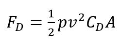
Typical aerodynamic drag coefficients (CD) for container ships range from 0.6 to 0.8 due to their bluff shape (Nguyen et al., 2016). Therefore, even moderate wind speeds can result in kilonewtons of drag. Since engine power rises to counter drag, reducing drag directly improves fuel efficiency and emissions performance (Xu et al., 2022).

Shipping accounts for about 3% of global CO₂ emissions (Fourth IMO GHG Study, 2020). With expanding global trade, this could increase substantially. Reducing aerodynamic drag plays a significant role in decarbonisation efforts. Reducing engine demand, enabling fuel savings, therefore complementing broader energy-efficiency strategies.

The Stern Wake Problem and Research Gap

Despite progress at the bow and midsection of the ship, the stern region remains under-researched.

Unlike road vehicles where rear-end shaping is crucial, ship design has largely overlooked the aerodynamic wake.

Few studies have explored rear drag-reduction devices. Van Nguyen et al. (2016) is one exception, proposing a "back guide," as seen in figure 1, that could potentially reduce drag by ~18% in simulations. Experimental work, however, was limited.

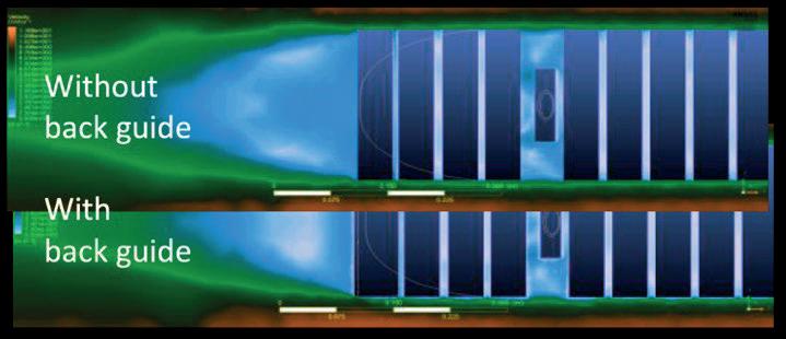
1: CFD data showing back guide potential wake reduction as seen through minor blue reduction on lower model (Source: Van Nguyen et al., 2016)

This study addresses that gap by testing a curved stern fairing to guide air smoothly off the structure. By controlling airflow from bow to stern, through the use of both a front cone and rear fairing, the aim is to manage separation throughout the ship's profile and reduce total drag.

Existing Drag Reduction Strategies

Many modern ship drag-reduction studies have focused on hydrodynamic improvements (Yang et al., 2013). Improved hull forms reduce wave and frictional resistance. Aerodynamics have been

significantly under-researched, leaving a gap in potential aid.

Ngô Văn Hệ et al. (2020) found that a sloped or rounded bow superstructure can reduce wind drag by ~30% compared to flat bows, as can be clearly visualised in figure 2. These cones deflect air upward, reducing stagnation zones. These designs are now used in car carriers and LNG tankers.

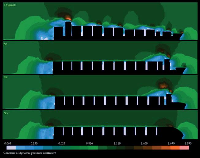
Figure 2: effect of front cone on frontal stagnation pressure (Source: Ngô Văn Hệ et al., 2020)

Other strategies include bow winglets, which generate vortices to guide air inward along the ship. Van Nguyen et al. (2016) again reported a 4–6% drag reduction using winglets on these vessels. Gap fillers between container rows have also shown to reduce internal turbulence.

Mathews’ (2024) front-mounted biomimicry design, inspired by the boxfish, featured a broad, angular frontal geometry aimed at reducing frontal drag. However, when applied, it disrupted airflow and caused greater flow separation. This led to the formation of a large, turbulent wake at the stern, as visualised by the large blue zone in figure 3, increasing aerodynamic drag. The present study seeks to address this issue by refining the ship’s profile, using a streamlined rear fairing in conjunction with this existing design.

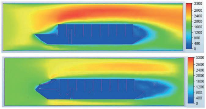
3: CFD analysis of traditional cargo vessel vs modified vessel with box-fish inspired nose cone

2024)

Fluid Dynamics Principles for Wake Control (Bernoulli and Coandă effects)

The fluid-dynamic principles behind this drag reduction are Bernoulli’s principle and the Coandă effect. Bernoulli’s principle explains that as a fluid's speed increases, its static pressure decreases, as can be visualised in figure 4. Therefore, drawing air over curved surfaces and preventing flow separation. By shaping the ship’s stern to encourage this smooth flow, the wake pressure is increased and pressure drag reduces (Xu et al., 2022)

The Coandă effect similarly describes a fluid’s tendency to follow a convex surface. As air flows over a curved stern attachment, the pressure on the convex side drops, drawing the flow toward the surface, delaying separation (Xu et al., 2022). This effect helps lower the wake and improve pressure loss and recovery.

Xu et al. (2022) demonstrated in LES simulations that forcing air along a convex surface can further reduce drag by keeping flow attached. They reported a 5.3–6.2% reduction in drag using this, as can be visualised in their findings in figure 5. These findings demonstrate that even passive curvature can reduce ship drag.

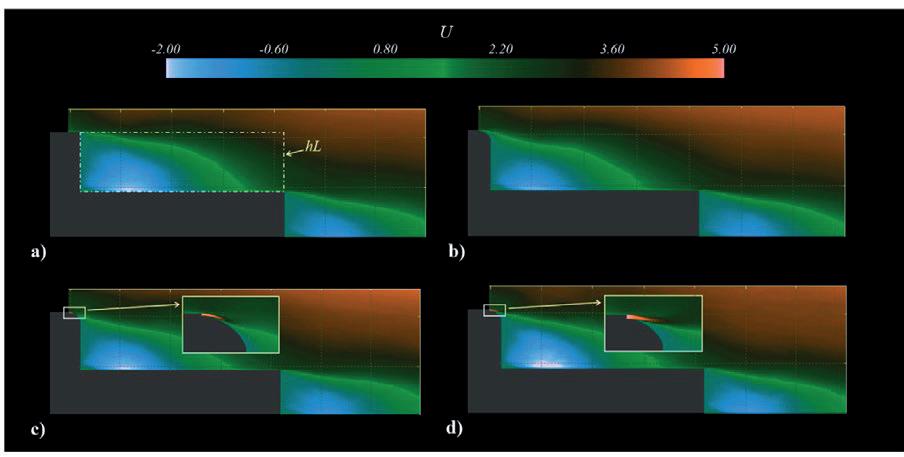
5: CFD data showing reduction in wake zone as a result of keeping flow attachment through the Coandă effect (Source: Xu et al., 2022)

Flow Separation, Wake Formation, and Pressure Drag

A large contributor to aerodynamic drag on large ships stems from pressure drag caused by flow separation (Wang et al., 2020). As air flows across the ship, it separates at straight edges. This separation forms a low-pressure wake where recirculating turbulent air reduces pressure. The front face experiences stagnation pressure, and the resulting high-to-low pressure gradient creates a net backward drag force (Wang et al., 2020).

Existing Wind tunnel and CFD simulations have visualised this: when flow separates from the rear of container stacks and off the back of the ship itself, it forms a large turbulent wake (Nguyen et al., 2016) as evidenced by the large blue section in figure 6.

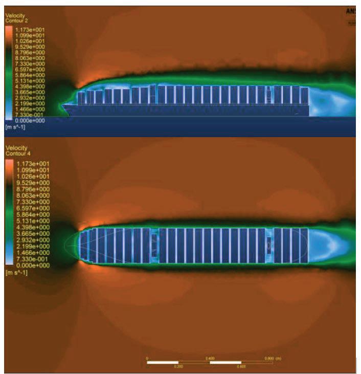
Additional studies show that tapered or streamlined cargo stacks reduce flow separation, raising wake pressure therefore reducing drag (Majidian & Azarsina, 2018). Conversely, uneven stacks increase drag by ~ 24% compared to optimised configurations

(Nguyen et al., 2016). Even uniform stacking increases resistance by 10% relative to tapered profiles (Hassan et al., 2012). These findings emphasise that wake control is essential to reducing aerodynamic drag.

Scientific Research Question

To what extent can a rear-mounted drag reduction system be employed to minimise aerodynamic drag force in the above-water structure of maritime freight carriers, alongside previously researched frontmounted drag reduction system?

Scientific Hypothesis

The application of a rear-mounted drag reduction system on maritime freight carriers will reduce aerodynamic drag both with and without a frontmounted drag reduction system.

Methodology

The investigation was conducted in three phases: (1) Design and fabrication of scale ship models with varying drag-reduction modifications, (2) CFD simulations to visualise flow and estimate potential, and (3) Wind tunnel experimentation to measure drag forces on physical models. This approach mirrors that of Mathews (2024) however focusses primarily on the stern drag reduction device.

A baseline 3D model of a 15,000 TEU post-Panamax container ship was developed using Autodesk Fusion 360 at a scale of 1:1000. This model included only the above-water superstructure, comprising the upper hull and stacked containers, shown in figure 7, designed to capture the geometry responsible for aerodynamic drag. Minimal underwater structure was included, both to reduce the effect of pre-designed hydrodynamic structures and to accommodate the wind tunnel mounting.

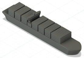
Figure 7: Traditional cargo vessel, modelled in Fusion 360.

Aerodynamic modifications were then developed and applied. Three rear-mounted drag-reduction systems were designed and attached individually to the stern of

an unmodified model. These consisted of convex faces, each angled downwards from vertical at 15°, 30°, and 40°, respectively, as shown in figure 8. Each segment extending approximately 10% of the ship’s scaled length.

An additional frontal modification, a box fish nose cone derived from Mathews (2024), was also implemented, as can be viewed in figure 9. This replaced the ship’s flat bow with a sloped structure intended to reduce frontal stagnation pressure.

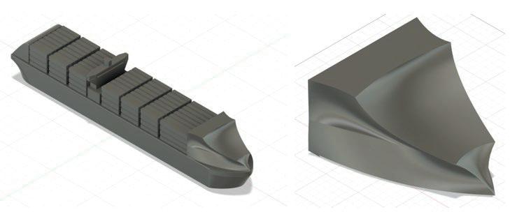
9: Cargo vessel with both front and rear modifications attached.

All configurations (baseline, nose only, and three rear fairings) were 3D printed using PLA at high resolution. The model featured a central mounting stub for force testing and maintained identical crosssectional area to allow correct drag coefficient comparison.

Figure 10: Three 3D printed rear mounted fairings with comparison to traditional vessel rear.

Part 2: CFD Simulation (Virtual

Wind Tunnel)

Computational Fluid Dynamics (CFD) simulations were conducted using Autodesk Fusion CFD to analyse airflow patterns on each ship model.

A virtual wind tunnel was constructed around each model. The domain dimensions extended to approximately five times the ship's length in all directions, ensuring that boundary proximity did not interfere with the flow behaviour. A laminar airflow velocity was applied at the front of the ship, corresponding to a wind speed of 30 km/h.

Each model was processed using automated meshing tools that concentrated detail around surfaces where flow separation and pressure gradients were most likely to occur. While airflow over the models would involve turbulent or varying behaviour at higher speeds or in real world scenarios, simulations were run under laminar flow assumptions due to software constraints and under the objective of capturing general aerodynamic trends.

The CFD solver ran 100 iterations, with flow stabilising at approximately 50 (figure 11), at which point flow field visualisations could be extracted for analysis.

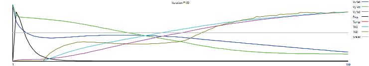
11: Fusion CFD convergence plot showing stabilisation across 100 iterations.

Part 3: Wind Tunnel Experimentation

A closed-circuit wind tunnel was employed to measure aerodynamic drag on scale ship models. The wind tunnel was adapted from one used by Mathews (2024). It includes a test section with internal dimensions of approximately 30 cm × 30 cm in crosssection and 80 cm in length, capable of housing the scaled ship models while minimising blockage effects.

The inlet of the tunnel featured a 3D-printed bellmouth intake designed to smoothly accelerate incoming air, reducing turbulence. A honeycomb flow straightener within the inlet ensures a laminar velocity flow before air enters the test section, as seen in figure 13. At the outlet, a 300 mm industrial axial fan drew air through the tunnel, configured in a suction-based layout to maintain steady airflow.

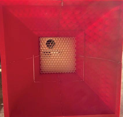
A variable autotransformer (240 V rheostat) was used to adjust fan speed. Wind speed inside the test section was measured in real-time using a digital anemometer mounted at the inlet of the tunnel. Each model was tested at velocities of 5, 10, 15, 20, and 25 km/h, each stabilised to within ±0.2 km/h. The ground plane was left solid, simulating air effect over water surface. This controlled, repeatable setup allowed consistent aerodynamic conditions for all models.

Testing

Drag force measurements were taken using a 1 kgcapacity strain gauge load cell mounted beneath the wind tunnel. A vertical support column connected the load cell to the ship model, passing through a small hole in the tunnel floor. This configuration isolated horizontal force along the wind direction. Load cell

Results

data was captured using an Arduino, as seen wired in figure 14. Prior to each test, the system was tarecalibrated to zero to negate the model’s static weight and any signal bias.

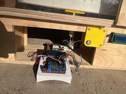
Testing involved positioning each ship variant onto the support plate. The wind tunnel was sealed, airflow was initiated and tuned to the desired speed, and a 60second stabilisation period was observed. Once airflow was steady, drag readings were recorded. For each wind speed and model configuration, three independent trials were conducted to ensure reliability. The model was removed and repositioned between trials to account for potential variability in alignment. All experimental conditions aside from the model design were held constant throughout.

Larger data is equivalent to a larger drag force on the ship. The darker green the data the better the model performed by producing less drag force, the darker orange the data the worst the model performed by producing more drag force.

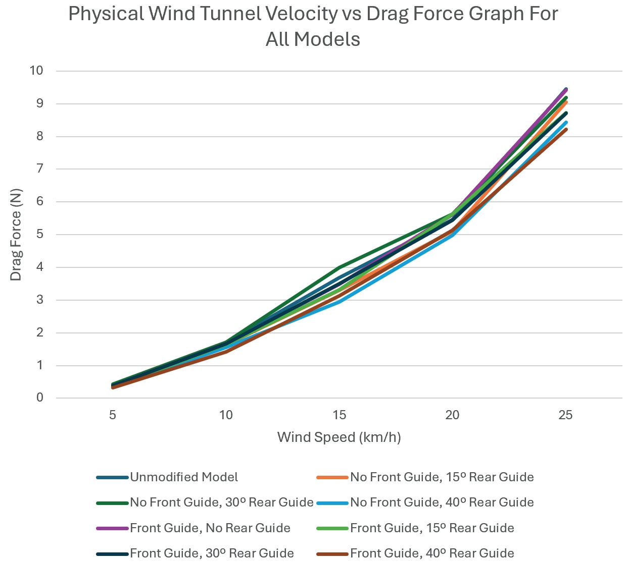
15: Wind velocity (km/h) vs drag force (N) graph of all models.

From this point results analysed primarily reflect data collected comparing the traditional unmodified cargo ship with the most efficient model (front guide and 40º rear guide), these have been chosen as they produced the highest and lowest average drag forces as seen in table 1. Additionally, the ‘front guide, no rear guide’ has been included for comparison. All other data regarding the remaining two back guides has not been referenced and has been placed in Appendix 1

Table 2: Comparison of unmodified model vs most efficient modified model (front guide and 40º rear guide) (mean data presented).

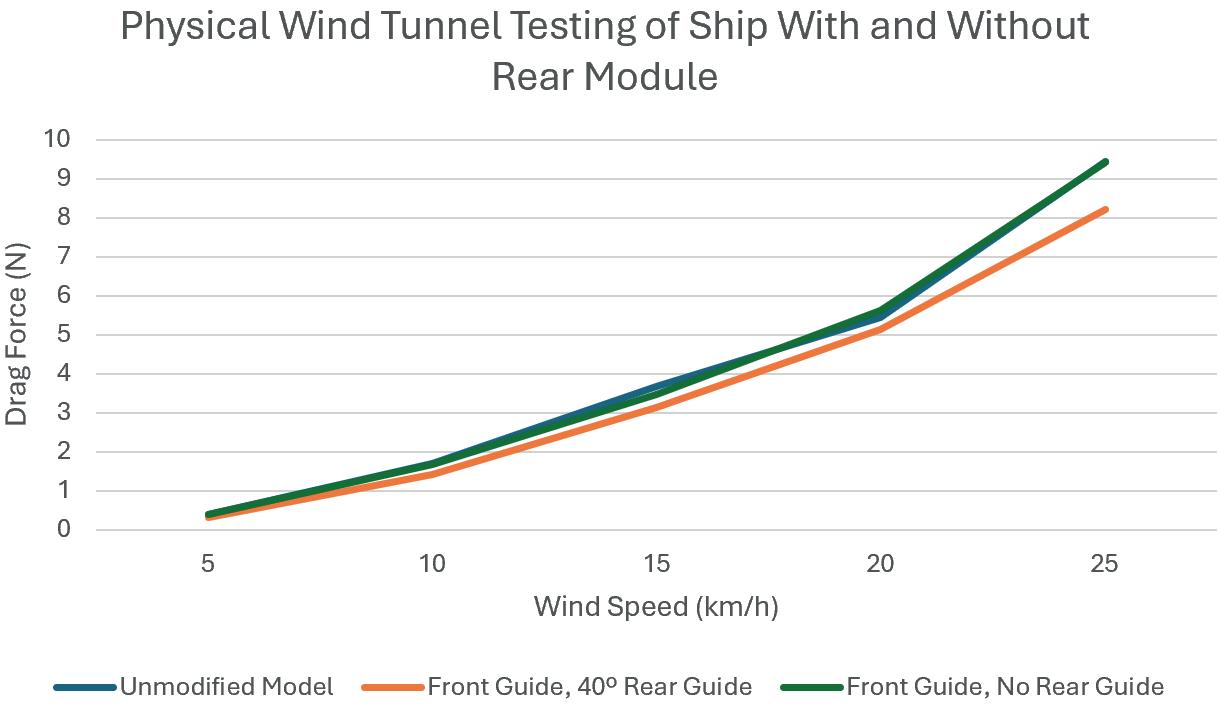
16: Graph (wind speed (km/h) vs mean drag force (N)) of unmodified model vs model with front guide and 40º rear guide in physical wind tunnel testing (‘front module, no rear module’ has also been added for comparison).

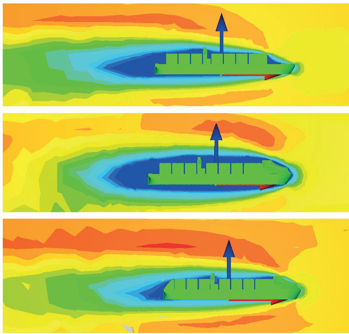
17: CFD pressure maps of unmodified model, front only model, and front + 40º rear attachment model showing wake reduction.

Discussion

Drag Force Measurements and Trends

Wind tunnel testing demonstrated a consistent reduction in drag force when comparing the unmodified ship configuration to the optimised design with both a frontal cone and a 40° rear fairing, as seen by the curve in figure 16. Mean drag forces were calculated for each wind speed, revealing that at all conditions tested, the modified model experienced lower aerodynamic resistance.

At the lowest speed tested (5 km/h), the average drag for the baseline was 0.397 N, while the modified model yielded 0.318 N, a reduction of ~20%. As wind speed increased, so did the absolute drag force on both models, however the modified variant consistently maintained lower values. At 25 km/h, the unmodified model reached 9.45 N, while the optimised model read 8.21 N, a decrease of only 13% (table 2).

This trend supports the expected quadratic relationship between velocity and drag, as outlined by the equation 1, however does suggest an experimental error within the testing setup as the reduction decreased by 7% as speed increased (table 2).

The increasing divergence in drag force values with speed supports the hypothesis that aerodynamic improvements are most effective under high-flow conditions. The plot in Figure 16 illustrates this widening gap, underscoring the performance benefit of streamlining.

Hypothesis Evaluation

The collected data supports the claim that there is a reduction of drag force through the use of a frontal and rear drag reduction system. At each increment, the optimised model outperformed the baseline. These results validate the aerodynamic benefit of modifying the stern edge of a ship’s profile.

Such outcomes are consistent with previous findings in similar domains, including land vehicles and civil transport. This also supports Nguyen et al.’s (2016) predicted reduction in ship drag through stern optimisation. This study builds on that foundation with physical testing, confirming those theoretical improvements under real airflow conditions.

Statistical Significance

To assess whether the observed difference in drag coefficients at 25 km/h was statistically significant, a two-sample t-test was conducted. The unmodified model yielded a mean drag coefficient of Cd = 0.320, while the modified model achieved Cd = 0.278. The calculated t-value was 3.49, resulting in a p-value of 0.025. Therefore, the difference is statistically significant with 95% certainty. This validates that this reduction in drag coefficient reflects a real, repeatable aerodynamic benefit under controlled wind tunnel conditions. These results support the conclusion that the combined modifications produce a reliable decrease in aerodynamic drag, however perform stronger in low wind conditions as opposed to higher wind scenarios where such improvements are most needed. These results were however additionally confirmed to be significant at all wind speeds.

Flow Field Analysis (CFD Insights)

The CFD simulations provide a visualisation of the drag reduction. Figure 17 shows side-by-side flow snapshots for the unmodified vs. modified configurations, additionally compared to Mathews' existing nose structure on the baseline model. In the baseline ship, as the air flows over the flat-topped, flat-backed geometry, a large low-pressure

wake forms immediately aft of the ship, in addition to the high pressure at the front of the ship. This is amplified using Mathews' design. This wake is depicted by an expansive blue region in the pressure contour. The wake’s low pressure effectively pulls backward on the stern, creating significant pressure drag (Mathews, 2024).

In contrast, the modified ship exhibits a markedly different flow pattern. The front cone guides the oncoming air up and over without separation at the bow, reducing the stagnation high-pressure zone on the front face. The rear fairing provides a convex surface for the air to follow at the stern. CFD shows that much of the airflow remains attached along the fairing, converging toward the water before shedding off, exiting the ship’s surface at a narrower angle than it does off the unmodified’s blunt end. This fills in the void that would otherwise become a low-pressure wake. This leads to a higher base pressure on the aft end of the ship, greatly reducing overall drag.

Comparison with Previous Work

These findings reinforce and extend previous research in several ways. Firstly, confirming the warning from Mathews (2024) that a bow-only biomimetic shape does not guarantee drag reduction. The large wake issue she found has been effectively addressed in this study by the addition of the stern fairing. This project implemented her suggestion and experimentally validated it. Leading to a significant drag decrease, indicates that her secondary hypothesis (that the boxfish design needed a complementary stern device) was correct.

Implications for Ship Design

The fairing is conceptually simple and can be retrofitted to existing ships. Mounted at the aft end of the final container stack, it deals only with airflow, not hydrodynamic loads, making its structural demands far less than a hull redesign. It can be constructed from lightweight materials, such as composites or steel shells, and tailored to avoid interfering with container handling or bridge visibility. Its ease of implementation makes it suitable for integration into the current fleet without major structural modification.

Limitations and Further Research

While results are successful, several limitations must be acknowledged:

Scale and Reynolds number effects

The wind tunnel tests were conducted at model scale and lower Reynolds numbers than those experienced by full-size ships. Though efforts were made to maintain dynamic similarity, effects such as

turbulence levels and effect due to material density will vary at full scale. Further CFD studies at higher Reynolds numbers, or full-scale field testing, would help validate the observed benefits, however, would be far more expensive.

Wind Angle Considerations

Tests focused exclusively on head-on wind, represent a worst-case scenario for aerodynamic resistance. However, real ships encounter wind from multiple directions. The additions performance under crosswinds remains uncertain, it may offer reduced benefits or even generate side force due to increased surface area. Future studies should evaluate how the fairing performs under various yaw angles and whether it could be shaped to streamline air from oblique directions.

Future Directions

Further research could refine the fairing’s geometry to optimise drag reduction without increasing complexity. Parameters such as curvature, taper angle, and length could be varied in CFD or wind tunnel studies. Additionally, applying this concept to different vessel types, such as cruise ships or vehicle carriers, could reveal even greater efficiency improvements due to their larger above-water profiles. With appropriate engineering, stern fairings may form part of a new standard in ship aerodynamic design

Conclusion

This investigation demonstrates that the addition of a rear-mounted drag reduction system, particularly when combined with a front-mounted nose cone, can meaningfully reduce aerodynamic drag on large container ships. Both CFD simulations and wind tunnel testing confirmed that the modified ship configuration consistently experienced lower drag forces than the unmodified baseline. The rear fairing effectively mitigated the formation of a large, lowpressure wake at the stern, while the front cone reduced the stagnation pressure at the bow. The combined design created smoother airflow from bow to stern, reducing flow separation and lowering the pressure differential across the ship, reducing overall drag.

Acknowledgements

I would like to thank Dr Matthew Hill for his guidance and support throughout this research paper. I would also like to thank Mr Phil Barden and the Design and Technology Department for their aid in the development and use of the physical wind tunnel.

References

Andersen, I. M. V. (2013). Wind loads on post-panamax container ship. Ocean Engineering, 58, 115–134. https://doi.org/10.1016/j.oceaneng.2012.10.008

Fourth IMO GHG Study 2020 Executive-Summary.pdf (n.d.). Retrieved February 10, 2025, from https://wwwcdn.imo.org/localresources/en/OurWork/Envir onment/Documents/Fourth%20IMO%20GHG%20Study% 202020%20Executive-Summary.pdf

Hassan, K., White, M. F., & Ciorta, C. (2012). Effect of Container Stack Arrangements on the Power Optimization of a Container Ship. Journal of Ship Production and Design, 28(01), 10–19. https://doi.org/10.5957/jspd.2012.28.1.10

He, N. V., Hien, N. V., Truong, V.-T., & Bui, N.-T. (2020). Interaction Effect between Hull and Accommodation on Wind Drag Acting on a Container Ship. Journal of Marine Science and Engineering, 8(11), Article 11. https://doi.org/10.3390/jmse8110930

Majidian, H., & Azarsina, F. (2018). Aerodynamic Simulation of A Containership to Evaluate Cargo Configuration Effect on Frontal Wind Loads. China Ocean Engineering, 32(2), 196–205. https://doi.org/10.1007/s13344-018-0021-1

Nguyen, T. V., Shimizu, N., Kinugawa, A., & Yoshiho, I. (2016). 2016A-GS18-10 Studies on Air Resistance Reduction Methods for a Large Container Ship (Part 1) 427–432. https://doi.org/10.14856/conf.23.0_427

Wang, P., Wang, F., & Chen, Z. (2020). Investigation on aerodynamic performance of luxury cruise ship. Ocean Engineering, 213, 107790. https://doi.org/10.1016/j.oceaneng.2020.107790

Xu, K., Su, X., Bensow, R., & Krajnovic, S. (2022). Drag reduction of ship airflow using steady Coanda effect. Ocean Engineering, 266, 113051. https://doi.org/10.1016/j.oceaneng.2022.113051

Yang, C., Huang, F., & Noblesse, F. (2013). Practical evaluation of the drag of a ship for design and optimization. Journal of Hydrodynamics, 25(5), 645–654. https://doi.org/10.1016/S1001-6058(13)60409-6

Appendix 1: Full physical wind tunnel testing table including all data from all testing.

Affluence and Mobility: Investigating traffic volume changes in Sydney during the 2020 and 2021 COVID-19 Lockdowns

Roy Yan Barker College

In response to the COVID-19 pandemic, the government of New South Wales, Australia, enforced restrictions on people’s movement, commonly referred to as “lockdowns”. These occurred in both 2020 and 2021 and had many varied impacts on the city of Sydney. To examine changes to traffic patterns, this research first draws upon literature as to how traffic in other cities changes due to similar restrictions before analysing secondary traffic flow data to answer the research question “How did a location’s affluence influence the magnitude of traffic volume reductions during the April 2020 and June 2021 COVID-19 lockdowns in Greater Sydney?”. Affluence was defined by median weekly household income, median weekly rent, and percentage of population holding bachelor’s degree or higher, and data for 24 different Local Government Areas was sourced from the ABS during the 2021 census. A definition for traffic volume reduction was developed through a case study of traffic data sourced from Transport for NSW traffic volume viewer about one location, Galston Road in the North-West of Sydney. Results in the first lockdown exhibited a weak positive correlation between affluence and traffic reduction, consistent with arguments posed in the literature that areas of greater affluence were able to reduce movement through increased ability to work remotely. However, this trend was reversed and weakened in the second 2021 lockdown where a slight positive correlation was observed. The research highlights how these restrictions have affected different communities and reinforces the need for policymakers to take these impacts into account.

Literature Review

Traffic Patterns in Sydney, Australia (Prior to COVID-19)

Sydney traffic conditions exhibit high levels of congestion compared to other cities, resulting from Sydney’s growing population and increased car ownership, with 1.75 cars per household (Trendle, 2019). According to the NSW EPA, the 6.2 million residents of greater Sydney, made 12 million daily journeys by car, roughly 2 per day for the average person (NSW EPA, 2021). Private vehicles dominated, accounting for around 67% of all Vehicle Kilometers Traveled (Corpuz, 2009). Sydney’s car reliance is reflected in low public transport usage, where it only accounted for 19.8% of daily journeys (Trendle, 2019). Traffic congestion is higher in peak hours, driven by commuter flows from outer suburbs into the central business district (CBD), but more recently Parramatta as a second CBD in the west (Glover & Dufty-Jones, 2022). From 2017 onwards to before the pandemic, passenger vehicle traffic was rising steadily at 1%, furthering traffic flows during peak hour (NSW EPA, 2018).

Impact of COVID-19 on Sydney

The outbreak global, of SARS-CoV-2, (COVID 19), was reported to have led to a substantial reduction in traffic in all areas of Sydney (Graham, 2020).

Key moments included the introduction of citywide stay-at-home orders on the 26/6/2021, in response to the Delta variant spread, with further unprecedented restrictions including a 10km travel barrier imposed on 5/7/2021 in the greater Sydney areas (Graham, 2020). Businesses were forced to adopt remote work arrangements, as well reduced spending opportunities for consumers, providing less of an incentive for residents to leave their homes (NSW Health, 2021). Other effects included a reduction in fuel consumption, road crashes and emissions, with the number of incidents falling by 50% and 60% in the first and second lockdown respectively (Chand et al., 2021).

Peak-hour congestion was eliminated during the period, with travel speeds increasing across major roadways. The NSW Government reported that by mid-2021 after lockdowns, travel times during traditionally congested periods had improved by up to 40% on key routes, including the M4 and M1 motorways. The Sydney Harbour bridge recorded

160,000 daily crossings before the pandemic, during the lockdown period, this fell to only 80,000, with an even more significant reduction in southbound traffic into the CBD during the morning peak, along with a redistribution in traffic, to other hours of the day (Uddin et al., 2022). However, this reduction in mobility was not equal across Sydney. Such as in areas with residents who had attained higher education and occupation levels, such as in Surry Hills, saw a more drastic drop in both April 2020 lockdown, and January 2022 reopening, with individuals in these areas showing more risk adverse behavior due to their ability to work at home, where the median λmob (logtransformed mobility ratio) in wealthier areas were lower, compared areas with lower education levels, where there was a more steady drop in mobility (Kollepara et al., 2024). Surry Hills, as recorded in the 2021 census has one of the highest rates of educational attainment nationwide, with 54.9% of the population holding a bachelor’s degree or higher, this is compared to the national average of 21.5% (ABS, 2021). Moreover, it held a median household weekly income of $2308, in comparison to the national median of $1746.

Many of occupations which were able to transition to remote work, include the finance, IT, and design industry (Reeson, 2021), reducing the need to commute, where Cheltenham had a decline in traffic between 6-8am of at least 70%, the time that corresponds to the highest volume of workers commuting into the CBD (Terrill, 2021).

Impact on other Cities

The outbreak of COVID-19 had a similar impact on traffic flows, including Milan and Manchester of 85% and 76% respectively (Merchant, 2020). New York, a city of 8.3 million was the worst area affected city in the United States and saw a drastic decrease in traffic flows in March 2020, of nearly 49% following the order on the 20th of March, to close all non-essential business (New York State, 2020). As expected, there was a drop in mobility, including on the subway, and usage of the cities ‘Citi Bikes’, with subway ridership dropping 95%, compared to 70% on cycling, with there being a sharper rebound in cycling, returning to pre-pandemic levels by September 2020, whereas subway ridership remained at 30% pre-pandemic levels (Wang & Noland, 2021).

Moreover, Data from the MTA (Metro Transit Authority) indicated a 68% drop in vehicular traffic via MTA bridges in April 2020 vs 2019, as well an increase in traffic speed of 108% on Midtown Avenues in NYC (Gao et al., 2020). However, the need for essential travel by lower-income workers in

blue collared jobs, could not work remotely, maintained higher-than-expected traffic levels in these communities (Liu & Stern, 2021). In the South Bronx and Harlem, where the median household income is $27,000–$29,000 USD, there was a 4.2% decrease in traffic, compared to lower Manhattan, with a 7.8% decrease, where the median household income is $138,000 - $160,000 USD (Statistical Atlas, 2018) This may be explained by higher income residents holding jobs where they are able to work from home, compared to lower income areas, whose residents may not have the ability to work from home (Shearston et al., 2024).

A trend that was observed in the third lockdown in the UK in January 2021, was mobility in more wealthy areas fell to just under 20% of pre-pandemic levels, compared to 10% in the first lockdown in London and Birmingham (Manthorpe, 2021). During the third lockdown, compliance among higher-income individuals was lower, with 9% of this group failing to isolate, potentially contributing to the smaller reduction in movement observed (Fancourt, 2021)

Scientific Research Question

How did a location’s affluence influence the magnitude of traffic volume reductions during the April 2020 and June 2021 COVID-19 lockdowns in Greater Sydney?

Scientific Hypothesis

More affluent suburbs in Greater Sydney will have experienced earlier and more substantial reductions in traffic volumes during the April 2020 and June 2021 COVID-19 lockdowns, compared to suburbs with lower median household incomes.

Methodology

Affluence of a LGA will be measured across three characteristics, (defined by higher median household incomes, higher education qualifications, and percentage of households that own their own dwelling). Traffic volume will be measured using publicly available Transport for NSW (TfNSW) traffic flow data. To establish a methodology for determining changes in traffic flow, initially the experiment looked at Galston Road in Hornsby.

The Raw Data

The secondary data was sourced from Transport for NSW traffic data viewer which collects raw traffic data from 600 permanent or temporary roadside collection stations. When analysing Galston Road, the process involved downloading the data from the

TfNSW database and importing it into an excel file. The data available included the amount of vehicle passing each hour, as well allowed it to be separated by direction, and heavy or light vehicles (Figure 1).

Figure 1: Traffic Volume Viewer Interface for Galston Road (Source: Transport.nsw.gov.au).

It was observed that there were missing values at some points of the day, over a few hour periods and over days, weeks, months potentially due to road closures or downtime for traffic sensors. There were also sometimes when the traffic flow would drop to a much lower percentage of the total amount on weekends and public holidays. The data was also downloadable as daily and weekly totals. These were simply a sum of all the values in that period which did not consider missing data, road closures, weekends, or public holidays. These all presented issues for analysis that needed to be considered.

Data Cleansing

The secondary data contained inconsistencies and inaccuracies and hence necessitated extensive data cleansing to ensure validity, and trends were able to be compared. It was determined that only daytime traffic (5 am – 11 pm) would be analysed, as this period best reflects community movement such as commuting.

Outside of these hours, traffic is typically limited to essential travel, and data may be unreliable due to nonoperational collection stations, reducing the accuracy of any measured changes. Similarly, weekends and public holidays were eliminated due to different patterns of traffic within the times with less commuter traffic during those times. Residents do not generally follow routine work or school travel behavior and is more recreational and dispersed across the day. Hence doesn’t represent standard commuter patterns.

Several gaps in the data were identified, potentially caused by either abrupt drops in traffic due to changing conditions or by non-operational data collection stations. If two or more such anomalies occurred within a single day, that day’s data was excluded from analysis. To account for this, the total number of days included in the weekly average was adjusted accordingly, reducing distortion of overall trends. This approach allowed for a small margin of error each day, ensuring that an excessive number of values were not excluded from the weekly analysis. From these weekly averages could be found, which was defined as the average number of vehicles per day between Monday and Friday.

Visualising Weekly Weekday Traffic Flow

From the cleansed data, it was possible to be able to plot weekly traffic volume over time (Figure 2). In the case of Galston Road, a 24-month baseline trend was able to be seen, as well the impact of the pandemic on movement.

Defining Average Traffic Before Lockdowns

From this data, decisions needed to be made as to how to define average daily traffic flow before the first lockdown. The immediate week before the lockdown

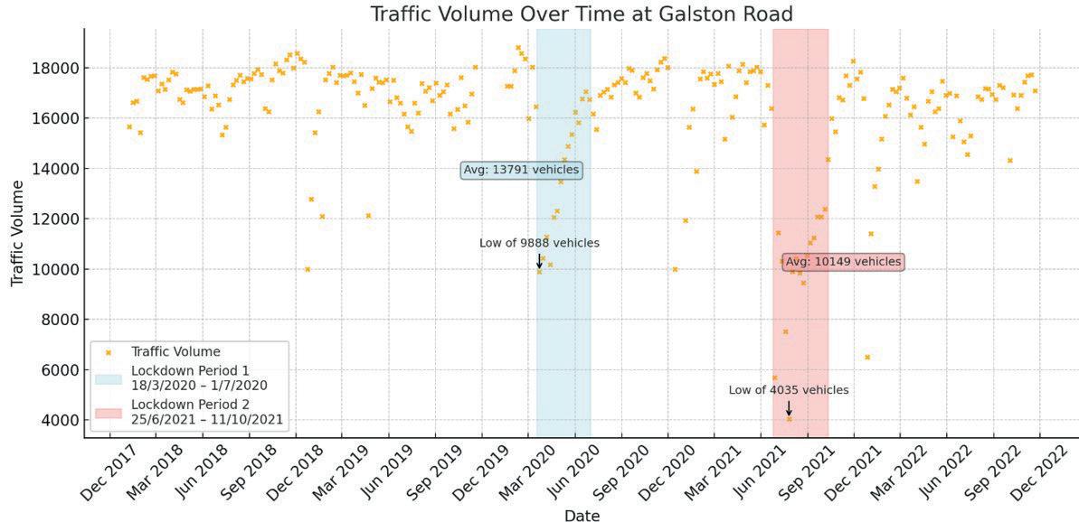
(starting 9/3/2020) there we 16959 cars passing Galston Road city-bound each day. However, the two weeks before that there were 18031, and 15990 cars respectively. Clearly taking the daily average for one random week in time was insufficient to accurately describe traffic before lockdowns were announced. Therefore, it was decided that a two-year (24 month) average would be taken to minimise the effect of random errors and predictable effects including seasonal trends, such as increased movement during summer months and school holidays. This baseline was used for the second lockdown as well. From the 24-month average it was deemed that daily traffic on Galston Road was 16959 cars. This is close to the value had the week immediately preceding lockdown been taken, however this can’t be assumed for all locations.

Defining Average Traffic Resulting of Lockdowns

Due to the abrupt shift in traffic patterns, establishing long-term trends proved challenging. As a result, the average daily traffic for each day during the first two weeks of both lockdowns was selected for analysis, as this period typically exhibited the lowest traffic volumes across the entire lockdown duration.

Defining Reduction in Traffic Volume

Reduction in traffic volume thus can be measured by comparing both the average of the first and second week separately each lockdown, to the pre-established 24-month baselines. Hence the percentage drop was able to be calculated (Equation 1).

Equation 1: Percentage Drop Formula

Application to Multiple Locations

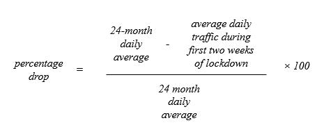
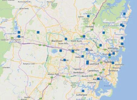
From this, 22 additional sites across greater Sydney were chosen, which met certain criteria, such as eliminating sites on major arterial roads, with a significant amount of non-local traffic, such as the M1 Pacific Highway site in Mooney Mooney. Moreover, the sites must’ve not had an extended period of nonoperation (greater than a month) in the 24 months prior, for a proper baseline to be established.

Analysis Methodology

To facilitate the efficient analysis of 24 traffic monitoring sites, a standardised methodology was developed. A uniform spreadsheet template was designed, with individual workbooks allocated to each site to enable consistent data processing. This structure allowed for automated data importation and cleansing, with embedded Excel functions applied systematically across all datasets. These spreadsheets were designed to display weekly averages and automatically refine the data to establish a consistent 24-month baseline. All site-specific data were then consolidated into a central spreadsheet, which generated key statistics including average vehicle volumes, baseline values for each site, and, most critically, the average percentage reduction in traffic volume for each site during the first two weeks of both lockdown periods.

This data would be compared with measures of affluence including median weekly rent, median weekly household income, and percentage with bachelor’s degree and above. The data was sourced from the ABS (Australian Bureau of Statistics) 2021 Census data, which allowed for data specific to each suburb. This ensured that the dependent variable (affluence), was able to be tested consistently in this experiment.

Results

During the first lockdown, there was a positive trend between affluence indicators, and drop in traffic. It was observed there was a weak positive correlation between income and traffic drop R² = 0.123, and an even weaker positive correlation between rent and traffic drop, R² = 0.043. However, the correlation between education and drop in traffic was nearly negligible, R² = 0.022. This trend was notably reversed or became more mixed in the second lockdown, with inconsistencies in the relationship between affluence and mobility reduction. A very positive weak trend was observed between median income and drop in traffic, R² = 0.007, while a weak negative trend was observed between median weekly rent and bachelor’s degree attainment, with R² = 0.029 and R² = 0.062 respectively.

Table 1 : Data on Drop in Traffic Flow from Baseline and Measures for Affluence for each Suburb Colour ed cells reveal the areas with the highest drop (lest traffic) in red, and the lowest drop (most traffic) in green.

Discussion

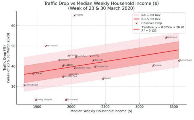
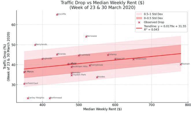
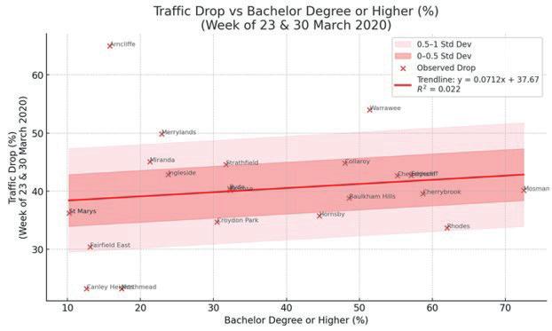
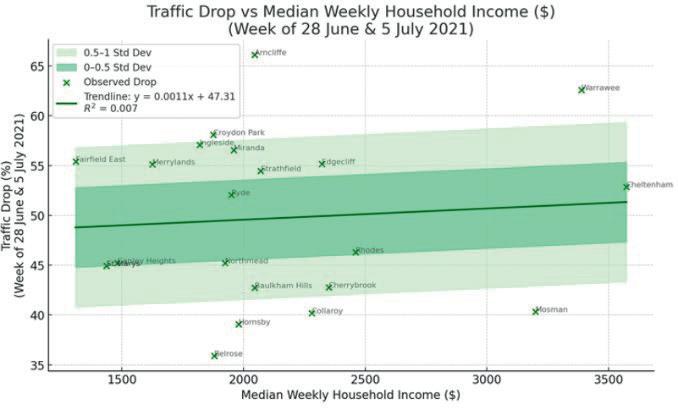
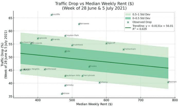
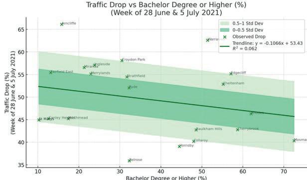
To better understand the changing relationship between affluence and mobility throughout the pandemic, case studies of various locations were undertaken to illustrate key suburban responses to lockdown measures.

Cheltenham

Cheltenham consistently lies close to the line of best fit across all six trendlines within 0.5 standard deviations and was therefore selected for case study analysis. It is a low-density residential suburb located 18km from the Sydney CBD in the Hornsby Shire, and high measures of affluence. Characterised in the 2021 census, where Cheltenham’s median rent was $695, 46% above the Sydney average of $475, and 55.2% of its population held a bachelor degree or above, compared to 33.9% of Sydney’s average (ABS, 2021). Within the first lockdown in the initial two week starting 23/3/2020 and 30/3/2020, it saw an average 42.6% drop, greater than other sites examined.

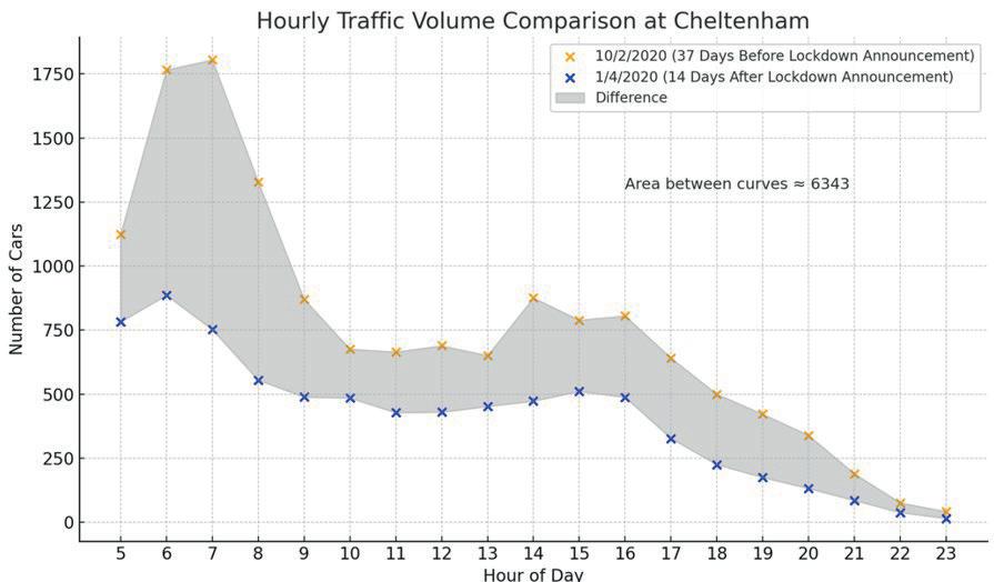
Cheltenham has 44.6% of its population working in professional industries, compared to the average of 25.8% in NSW (Australian Bureau of Statistics, 2021). This supports existing literature suggesting that more affluent communities exhibit greater mobility elasticity, enabling them to achieve larger reductions in traffic flow. At 8 am, during the morning peak period (Saunokonoko & Blancato, 2020), traffic volume decreased by 82%. This substantial reduction greater than that recorded in Fairfield indicates a pronounced decline in commuter activity and supports the inference that residents in this area had a greater capacity to work from home.

Fairfield East

Fairfield East consistently exhibited a relatively smaller reduction in traffic, ranking within the lowest 20% for traffic decline across all six-trend analysis. It’s a medium density community in the western suburbs 27km from the CBD of 5198 residents, is characterised by lower socioeconomic indicators. Where 12.1% of its population holds a bachelor’s

degree, a median rent of $364 and median weekly household income of $1092, which are all below the Sydney average.

Moreover a recommendation from the NSW Department of Education on the 24/3/2020 to keep students home and with 18.1% of Fairfield’s population being school age, may of contributed to a 54.5% drop between the hours of 7-9am (Figure 11) the peak time for school traffic (RAA, 2024)

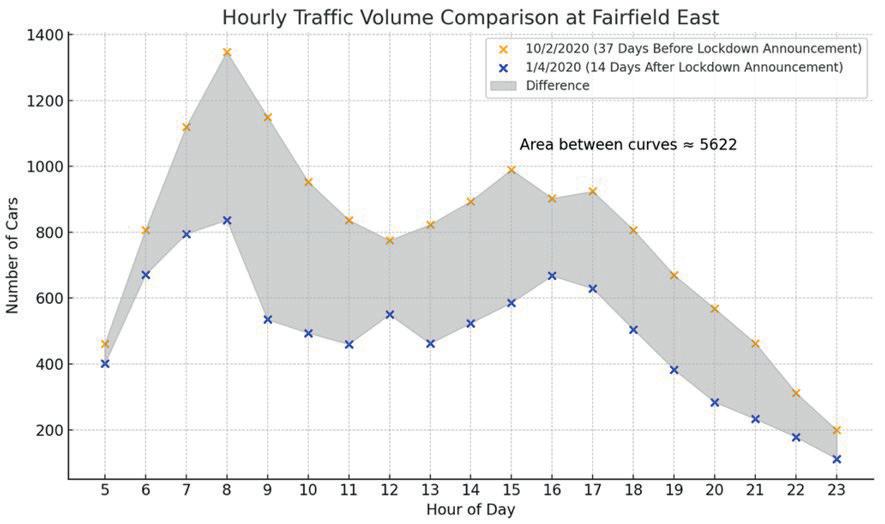
Figure 11: Hourly Traffic Comparison for Fairfield between Traffic on 10/2/2020 and 1/4/2020

Mosman

Mosman, a highly affluent suburb located 8km from the Sydney CBD, with average rent of $780 per week and 54.5% holding a bachelor’s degree or above, where it saw a lower reduction in the first week of 48% (Table 1). May have led to greater complacency and hence movement within the community. One theory is in more affluent areas, ‘pandemic fatigue’ set in earlier in wealthy areas, due to greater level of compliance in the first lockdown, leading to growing complacency in the second lockdown. As well, during the pandemic restrictions were applied inequitably across communities. On 23/8/2021 more intense restrictions for certain LGA’s including a curfew (Nguyen, 2021), which was applied predominantly in areas of low affluence, hence a further reduction in mobility.

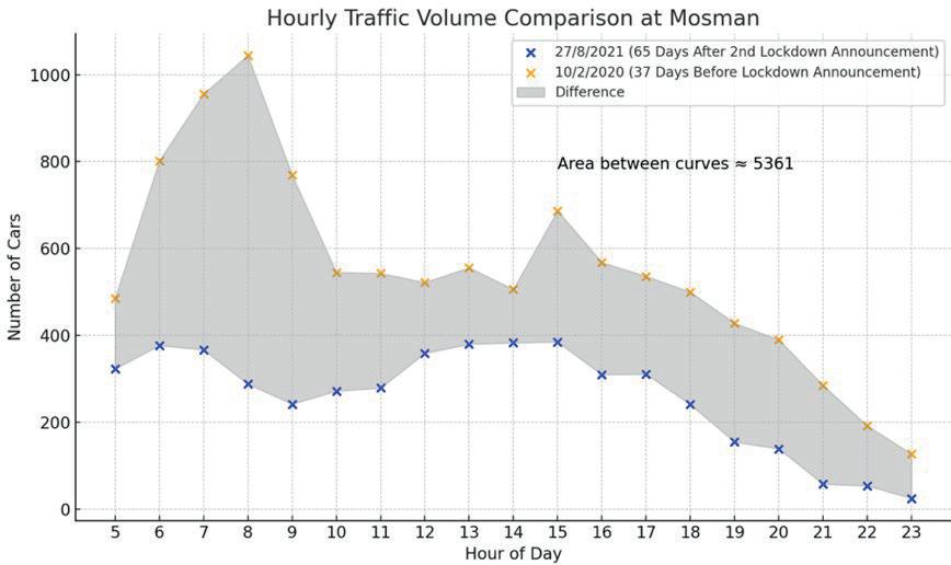
Figure 12: 13 Hourly Traffic Comparison for Mosman between 10/2/2020 and 27/8/2021

Arncliffe

Arncliffe was a site that was a consistent outlier in all 6 trend lines, being as much as 2.92 standard deviations from the trend line (Figure 8). This may be attributed to its proximity to lockdown affected travel zones, including Sydney Airport which had a 74.7% drop in passenger arrivals (Catterall & Clements, 2021), which lead to a potential greater drop in traffic.

Conclusion

The investigation found that affluent suburbs in Greater Sydney generally experienced larger and earlier reductions in traffic volumes during the first COVID-19 lockdown possibly partially supporting the original hypothesis. Case studies of Cheltenham and Fairfield East revealed varying nature of employment as a possible cause. However, in the second lockdown there was a weakening and reversal of the trend, where areas of lower affluence saw a greater drop in traffic, contradicting the hypothesis. The results may be able to be explained by trends proposed by the literature such as increased complacency among affluent households, where this correlation was found in Mosman where it experienced a smaller drop in traffic. Moreover, in both lockdowns, anomalies including Arncliffe highlight the influence of external factors on measuring movement.

Acknowledgements

Since starting this project in November of 2024, I’ve been privileged enough to work with Dr Matthew Hill, who has provided me with unwavering support throughout this project. His dedication to not only the subject, but my project as well has ensured that I’ve been able to deliver this report. His countless edits, advice and teachings have proven invaluable. I’d also like to thank my other Science Extension classmates, where they have supported me in keeping passionate and accountable over the course of my project.

References

ABS. (2021). 2021 Surry Hills, Census All persons QuickStats, Australian Bureau of Statistics https://abs.gov.au/census/find-censusdata/quickstats/2021/SAL13714

Australian Bureau of Statistics. (2021). 2021 Cheltenham (NSW), Census All persons QuickStats, Australian Bureau of Statistics https://abs.gov.au/census/find-censusdata/quickstats/2021/SAL10895

Catterall, R., & Clements, J. (2021). 2020_Full_Year_Results_Release. Sydney Airport. Chand, S., Yee, E., Abdulmajeed, A., & Vinayak, V. D. (2021). A Descriptive Analysis on the Impact of COVID-19 Lockdowns on Road Traffic Incidents in Sydney, Australia.

International Journal of Environmental Research and Public Health

City of Sydney. (2023, April 23). Economic snapshot shows city recovery, City of Sydney News https://news.cityofsydney.nsw.gov.au/articles/economicsnapshot-shows-city-recovery

Corpuz, G. (2009). Public Transport or Private Vehicle: Factors That Impact on Mode Choice. Australasian Transport Research Journal

Fancourt, D. (2021, January 21). Lockdown compliance improving but low take up of Covid tests ‘worrying’, Faculty of Population Health Sciences. https://www.ucl.ac.uk/population-healthsciences/news/2021/jan/lockdown-compliance-improvinglow-take-covid-tests-worrying

Gao, J., Wang, J., Bian, Z., Bernardes, S. D., Chen, Y., Bhattacharyya, A., Thambiran, S. S. M., Ozbay, K., Iyer, S., & Ban, X. J. (2020). The Effects of the COVID-19 Pandemic on Transportation Systems in New York City and Seattle, USA. C2 Smart

Glover, B. M., & Dufty-Jones, R. (2022). Parramatta 2035: Vibrant, Sustainable, Global. Centre for Western Sydney Graham, B. (2020, May 15). Staggering traffic figures reveal extent of lockdown https://www.9news.com.au/national/coronavirus-trafficdata-large-drop-in-congestion-during-covid19-lockdownexclusive/dce9c3eb-2b29-43f1-b083-28fc2c7caaf0?utm

Kollepara, Subhrasankha Dey, Martin Tomko, Erika Martino, Rebecca Bentley, Michele Tizzoni, Nicholas Geard, & Cameron Zachreson. (2024). Socioeconomic correlates of urban mobility trends in two Australian cities during transitional periods of the COVID-19 pandemic. R Soc Open Sci

Liu, Z., & Stern, R. (2021). Quantifying the Traffic Impacts of the COVID-19 Shutdown. Journal of Transportation Engineering, Part A: Systems, 147(5), 04021014. https://doi.org/10.1061/JTEPBS.0000527

Manthorpe, R. (2021, January 9). COVID-19: Lockdown data suggests people have become used to bending the rules Sky News. https://news.sky.com/story/covid-19-lockdownmobility-data-shows-people-have-become-accustomed-tobending-the-rules-12182919

Merchant, A. (2020, March 17). What Can Traffic Data Tell Us about the Impact of the Coronavirus? TomTom Newsroom https://www.tomtom.com/newsroom/explainers-andinsights/covid-19-traffic/

New York State. (2020, March 20). Governor Cuomo Signs the “New York State on PAUSE” Executive Order, Governor Kathy Hochul. New York Governor. https://www.governor.ny.gov/news/governor-cuomo-signsnew-york-state-pause-executive-order

Nguyen, K. (2021, August 20). Sydney lockdown extended for one month as NSW records 644 COVID-19 cases, four deaths ABC News https://www.abc.net.au/news/2021-0820/nsw-records-644-covid-19-cases-and-fourdeaths/100392702

NSW DoE. (2020, March 23). Restrictions begin as schools move towards online learning. Restrictions Begin as Schools Move towards Online Learning; NSW Department of Education. https://education.nsw.gov.au/news/latest-

news/restrictions-begin-as-schools-move-towards-onlinelearning.html

NSW EPA. (2018). Trends in Motor Vehicles and their Emissions

NSW EPA. (2021). Transport, NSW State of the Environment. https://www.soe.epa.nsw.gov.au/allthemes/human-settlement/transport

NSW Health. (2021). COVID-19 restrictions tightened across Greater Sydney. https://www.health.nsw.gov.au:443/news/Pages/20210709 _03.aspx

O’Sullivan, N. C., Matt. (2021, June 27). NSW records 30 new cases of COVID-19 on first day of Sydney’s lockdown [News Article]. The Sydney Morning Herald. https://www.smh.com.au/national/nsw/nsw-records-30new-cases-of-covid-19-on-first-day-of-sydney-s-lockdown20210627-p584l9.html

RAA. (2024, July 22). School pick-up the worst time of day for pedestrian crashes. RAA Daily. https://daily.raa.com.au/media-resources/school-pick-upthe-worst-time-of-day-for-pedestrian-crashes/?

Reeson, A. (2021). Staying connected Working, and socialising, from home during the COVID-19 pandemic

Ryan, G. (2021, August 15). Am I an essential worker? Find out here https://www.newcastleherald.com.au/story/7386494/am-ian-essential-worker-find-out-here/

Saunokonoko, M., & Blancato, T. (2020, August 25). Traffic hell: Top five congested roads in Sydney and Melbourne https://www.9news.com.au/national/top-five-worst-trafficroads-sydney-nsw-and-melbourne-victoria-tomtom-datarevealed/13b9b824-8b26-41b5-9b3f-b9abb4cfd5c4?

Schweizer, A.-M., Leiderer, A., & Mitterwallner, V. (2021). Outdoor cycling activity affected by COVID-19 related epidemic-control-decisions. PLoS

Shearston, J. A., Saxena, R., Casey, J. A., Kioumourtzoglou, M., & Hilpert, M. (2024). Variation in the Impact of New York on Pause on Traffic Congestion by Racialized Economic Segregation and Environmental Burden. GeoHealth, 8(12), e2024GH001050. https://doi.org/10.1029/2024GH001050

Statistical Atlas. (2018, September 14). The Demographic Statistical Atlas of the United States Statistical Atlas https://statisticalatlas.com/neighborhood/New-York/NewYork/South-Bronx/Household-Income?

Terrill, M. (2021, July 3). Stuck in traffic: Busting Melbourne versus Sydney myths and identifying the worst commutes. Grattan Institute https://grattan.edu.au/news/stuck-in-traffic-bustingmelbourne-versus-sydney-myths-and-identifying-theworst-commutes/

Trendle, B. (2019). Public transport access and its implications for household car ownership: A case study of the Sydney Greater Metropolitan. Australasian Journal of Regional Studies

Uddin, S., Khan, A., & Zhou, F. (2022). Road networks and socio-demographic factors to explore COVID-19 infection during its different waves. PubMed

Wang, H., & Noland, R. B. (2021). Bikeshare and subway ridership changes during the COVID-19 pandemic in New York City. Research Centre for Integrated Transport Innovation (rCITI), 106, 262–270. https://doi.org/10.1016/j.tranpol.2021.04.004

Biology and Earth & Environmental Science

This year, five students undertook fascinating research projects in the fields of Biology and Earth and Environmental Science. Their innovative work explored solutions to real-world problems.

Ally pursued her passion and investigated the ecological factors driving tool-use behaviour in wrasse species, providing valuable insights into the cognitive abilities and evolutionary adaptations of marine life. Bowen’s project reviewed available data to investigate geographic variation in the Eastern Brown snake venom. His analysis revealed limited but compelling evidence that the venom’s composition and yield differ based on location, highlighting the need for more research to improve snakebite treatment.

Melissa’s interest in plant biology led her to investigate how various treatments could prolong the colour stability of cut flowers. Her findings offering valuable insights for the commercial cut flower industry. Brett combined his passion for plant biology, agriculture, and environmental science to investigate a natural solution for agricultural pollution. His project successfully demonstrated that the native Australian plant Carex appressa is a highly effective biofilter, capable of removing phosphates and nitrates from simulated piggery runoff. His findings suggest a promising way to minimise the environmental impact of agriculture waste.

Eddy combined his passion for biology, agriculture, and software design to investigate the impact of modern farming practices on a vital pollinator. His project used AI-assisted video analysis to measure bee visitation rates to genetically modified canola fields treated with glyphosate. This novel approach of integrating software design with biological research demonstrates how interdisciplinary methods can provide new insights into complex environmental issues.

Does Glyphosate application affect pollinator visitation on Round-Up ready Tru-Flex Canola

Eddy Phillips Barker College

This study investigates the impact of glyphosate herbicide application on bee visitation rates in genetically modified (GM) Roundup Ready Tru-Flex canola (Brassica napus). Prior research has identified glyphosate as negatively affecting bee cognition and pollen quality, yet the specific effects on direct pollinator visitation to treated plants remain unexplored. Using controlled experimental plots, bees' visitation rates were measured through direct observation and AI-assisted video analysis following glyphosate application. Preliminary evidence suggests reduced bee visitation on glyphosate-treated canola, potentially attributed to altered pollen characteristics or cognitive impairment. Understanding these effects is vital for optimizing pollination and productivity in Australian canola agriculture.

Literature Review

Effect of Glyphosate on bees

Glyphosate-based herbicides, though not directly targeting insects, are increasingly linked to sub-lethal harm in bees. Honeybees (Apis mellifera) exposed to field-realistic doses of glyphosate show impaired cognitive functions such as reduced associative learning and memory, negatively impacting their foraging efficiency and navigation (Farina et al., 2019; Mengoni Goñalons & Farina, 2018). Even brief exposure can significantly weaken bees' olfactory learning, as evidenced by a reduced proboscis extension reflex to trained scents (Farina et al., 2019)

Beyond cognition, glyphosate exposure also causes various biological stresses in bees. A recent systematic review highlighted numerous sub-lethal impacts, including diminished foraging activity, slowed brood development, and disrupted gut microbiota (Tan et al., 2022). Glyphosate particularly reduces beneficial gut bacteria like Snodgrassella, increasing bees' vulnerability to pathogens and nutritional deficits (Farina et al., 2019; Motta et al., 2018). These physiological disruptions can indirectly lower bee survival and overall colony performance.

Additionally, glyphosate may affect pollinator behaviour indirectly by altering floral resources. Russo et al. (2023) found that herbicide treatments can reduce pollen and nectar nutritional quality (e.g., lowering amino acid concentrations), thereby decreasing insect visitation. Field experiments demonstrated a strong correlation between lower pollen quality due to glyphosate exposure and reduced pollinator visits, indicating that treated plants become less attractive or nutritious to bees. Despite these findings, direct field evidence of glyphosate's impact on bee visitation rates remains limited. This study

aims to address that gap by comparing pollinator activity in glyphosate-sprayed versus unsprayed canola, examining if herbicide-induced sub-lethal effects result in observable changes in visitation under agricultural conditions.

Economic importance of Canola

Pollinators are key to canola (Brassica napus) production, a major oilseed crop worldwide and in Australia. Canola is self-pollinating to a limited degree, but numerous experiments globally reveal that insect pollination (predominantly by honey bees) increases canola production and quality by a significant amount (“Pollination of Crops in Australia and New Zealand,” 2012). Bee visitations to flowers increase pods per plant and seeds per pod, and can increase seed weight and germination percentage (“Pollination of Crops in Australia and New Zealand,” 2012). For instance, experiments in farm fields showed that canola plots with high bee visiting had 15–20% higher rise in production compared to those with zero managed pollinators (“Pollination of Crops in Australia and New Zealand,” 2012). Australian canola production was worth AUD $6.6 billion during the 2022–23 season (Australian Agriculture, 2025). Pollinators add substantially to that through increases in crop yields. Catarino et al. (2019) showed that pollination frequently beats agrochemical inputs to boost oilseed crop profitability: plots with higher bee density across habitats recorded 15–40% higher yields and gross margins when compared with those with smaller pollinator counts (Catarino et al., 2019). This study’s focus on glyphosate effects on bee visitation addresses an important aspect of that balance for canola growers in Australia.

AI in Environmental monitoring and bee detection

Recent advances in artificial intelligence (AI) and machine learning have significantly enhanced wildlife monitoring capabilities, including pollinator studies.

AI-powered image recognition can efficiently process large datasets, automatically counting and tracking animals from camera traps and video footage, tasks typically tedious for manual observation (Bhuiyan et al., 2022; Spiesman et al., 2021) Specifically, deep learning models such as convolutional neural networks have demonstrated high accuracy in detecting bees from videos and tracking their movements. For instance, Bjerge et al. (2023) successfully used YOLOv5 models to detect bees with over 92% precision and recall, illustrating AI’s potential to achieve detailed, continuous monitoring previously unachievable by human observers alone.

However, practical application of AI in ecological monitoring faces notable challenges. Key among these is the necessity for extensive, high-quality annotated datasets. Limited datasets often result in poor model performance, characterized either by missed detections (low sensitivity) or false positives (low specificity), particularly when bees appear as small, fast-moving objects in complex and dynamic backgrounds (Bjerge et al., 2023; Kongsilp et al., 2024) Additionally, the "black box" nature of deep learning models presents interpretability challenges. Without explainable AI methods like saliency maps, it's difficult to verify whether detection differences between experimental conditions reflect genuine ecological variation or mere detection biases (Petsiuk et al., 2021).

Despite these constraints, AI-driven monitoring offers considerable promise. It provides continuous, noninvasive data collection and potentially real-time insights into pollinator dynamics and responses to agricultural practices. This study leverages these technologies to assess bee activity in glyphosatetreated canola, highlighting both their potential and the critical areas requiring improvement for broader ecological application.

A literature-based methodology

A core aim of our methodology was to use video recordings and AI-assisted analysis to efficiently monitor bee visitation, significantly reducing manual effort and increasing data accuracy. Traditional pollinator observation methods are labour-intensive, susceptible to observer fatigue and human error (Bhuiyan et al., 2022; Bjerge et al., 2023). By contrast, AI rapidly processes large datasets and consistently identifies pollinators over extended periods, greatly enhancing data quality even when resources are limited (Kongsilp et al., 2024; Spiesman et al., 2021)

The plot layout and experimental approach were inspired by AgriFutures Australia’s Clover4Bees

project, which used replicated small plots to systematically evaluate pollinator preferences under controlled conditions (“Pollination of Crops in Australia and New Zealand,” 2012). Similarly, we established discrete 1 m × 2 m plots comparing glyphosate-treated and untreated controls, enabling precise side-by-side comparisons. Glyphosate applications were carefully timed to avoid confounding variables like weather or spray drift, standard practices recommended in pollinator pesticide research to maintain treatment integrity (Vicens & Bosch, 2000). Additionally, plot observations were systematically rotated each sampling day to prevent bias from daily fluctuations in bee activity, aligning with established protocols that account for environmental variability (Vicens & Bosch, 2000). Midday observations were chosen deliberately, reflecting literature findings that honey bees exhibit peak foraging activity under warm and sunny conditions, further enhancing our data reliability (The Influence of Time of Day on the Foraging Behavior of the Honeybee, Apis Mellifera, 1989)

Thus, our experimental design integrates innovative AI methods (Bhuiyan et al., 2022; Petsiuk et al., 2021) with well-established field methodologies (“Pollination of Crops in Australia and New Zealand,” 2012; Vicens & Bosch, 2000) to robustly assess glyphosate’s impact on bee visitation.

Scientific Research Question

How does glyphosate herbicide application affect pollinator visitation and foraging behaviour in RoundUp Ready Tru-Flex canola? Can AI technologies reliably detect and quantify these changes?

Scientific Hypothesis

Canola treated with glyphosate herbicide will exhibit reduced bee visitation rates compared to untreated controls.

Methodology

Clear 3 identical 1m x 2m plots and plant Round-Up Ready, Tru-Flex Canola with a row spacing of 30cm and crop spacing of 10cm, adding two seeds into each hole at each interval, labelling them as plot 1, 2 and 3 in sequential order, keeping plot 3 as a control plot. Monitor growth until plants are close to first flower (50-90 days). 3-4 days before first flower, spray two adjacent plots, downwind from the control plot, spraying the base of each plant and any surrounding weeds individually, making sure there is no imminent rain until at least 60 minutes after spraying and

weather conditions, namely wind, are stable. 5-7 days after first spray (weather permitting), and after a small amount of floral emergence, respray plot 1 in the same manner detailed previously, making sure it is still downwind from the control plot. Take note of any floral abundance which may be in closer proximity to some plots than others and eliminate if possible. Setup monitoring cameras on two of the 3 plots, monitoring them every second day for 14 days (7 days of footage) between the times of 12pm and 1pm, switching which plots are monitored every filming session and downloading footage off the cameras on each nonfilming day. Separate the videos up into 5 separate parts (approximately 12 minutes long) and manually observe the footage making note of any bee that remains stationary and retracts its wings momentarily on a flower. Determine the 5-minute average counts for each video part as well as the 5-minute average counts for each individual plot. Run each 12-minute clip through each AI Model (AI 1, AI 2 and AI 3), to determine the accuracy of the models and attempt to confirm manual counts with a confidence threshold of > 0.5.

Results

Overview of data collection

Over the monitoring period, bee visitation to canola flowers was assessed under two treatment conditions: glyphosate-sprayed plots versus an unsprayed control plot. Bee counts were obtained through two methods, direct manual observations of video footage and AIdriven video analysis, until data collection was cut short by an unexpected disturbance. Midway through the experiment, an intrusion of sheep into the plots led to extensive grazing of the canola plants, especially in the treated areas. This incident occurred soon after the second day of observations and effectively compromised any further data collection. As a result, only the initial two days of data (prior to the sheep damage) were considered reliable and are presented here. While limited, these initial observations provide preliminary insights into visitation patterns.

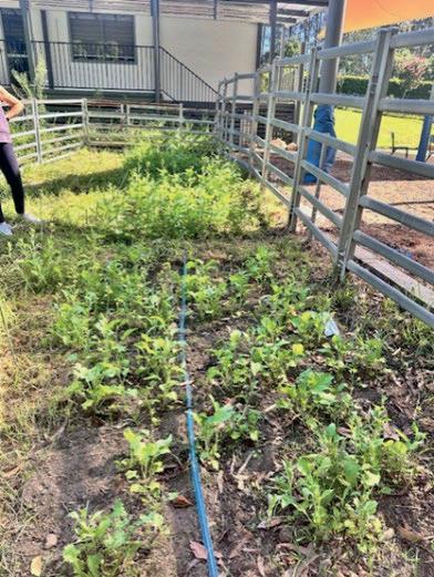
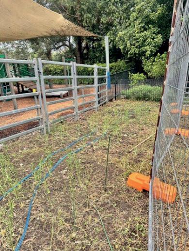
Direct observations

Table 1 below summarizes the bee visitation counts from human observations taken from video footage on two different dates (19th of March and 20th of March) across the plots. On the sunny day (19th March), the untreated control plot had higher bee visitation on average than the glyphosate-sprayed plot. On the following cloudy day, bee activity decreased markedly in both plots, and the visitation gap between

the control and treated plot narrowed. These results suggest a potential reduction in pollinator visitation associated with glyphosate treatment, though weather variability had a strong influence as well.

Table 1: Averaged direct observation bee counts

1

On Day 1 (March 19th), under sunny conditions, the glyphosate-treated plot averaged approximately 12.6 bee visits during the observation period, while the control plot (Plot 3) recorded a notably higher average of 17.9 visits, nearly 40% more activity. This changed dramatically on Day 2 (March 20th) when cloud cover moved in. Bee activity dropped sharply in both plots, with the treated plot averaging 10.7 visits and the control plot 10.3 visits, essentially eliminating the difference we'd observed the previous day.

AI Based detection results

The video footage from the control plot on the 19th of March was analysed with three iterations of AI models (referred to as AI Model 1, 2, and 3) to automatically detect and count bee landings. The raw detection counts from each model were compared against the manual counts for validation. A clear trend of improvement was observed across the three models, although each had limitations.

Table 2: AI Model counts

Model 1 (initial model): trained on 500 images, 53 of which contained bee visitations, vastly overestimated bee occurrences. For example, in the control plot’s Day 1 video, Model 1 registered 219 “bee” detections compared to the actual 34 bees counted.

Model 2 (second iteration): trained on 1000 images, 115 of which contained bee visitations, took a nearly opposite approach, severely under-counting bees. Using improved training data and stricter detection thresholds, Model 2 avoided the rampant false positives of its Model 1 but missed many real bee visits. In the same example segment, Model 2 detected only 5 of the 34.

Model 3 (third iteration): trained on 2000 images, 240 of which contained bee visitations, achieved a more balanced detection. Refinements to the algorithm and additional training examples helped Model 3 detect more of the actual bees while keeping false positives relatively low. In the example case, Model 3 identified 8 out of 34 bees, still an undercount, but better than Model 2’s 5, and with far fewer false positive detections than Model 1.

Discussion

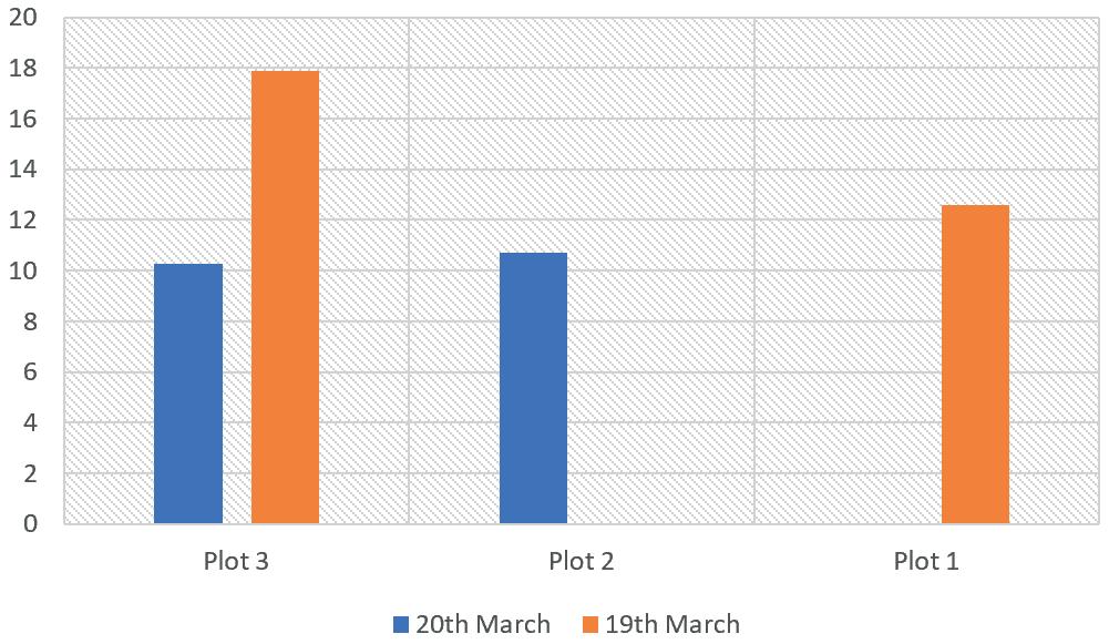
Weather and resource variability

The observations underscore the dominant influence of weather and floral resource availability on honeybee foraging activity. Bee visitation rates dropped drastically on the overcast Day 2 compared to the sunny Day 1, in both glyphosate-treated and control plots as shown in figure 1 above. This aligns with numerous studies showing that honey bees require warm temperatures and clear skies to forage optimally; they dramatically reduce flight activity under cool, cloudy, or windy conditions (Karbassioon et al., 2023; Vicens & Bosch, 2000). Vicens and Bosch (2000) recorded that foraging ceases almost entirely when temperatures fall below 15 °C or during rainfall, somewhat in line our Day 2 findings, suggesting the cause of the drop in visitation. Kunin (1997) demonstrated that even modest increases in floral density significantly boost bee visitation, explaining why the control plot, slightly richer in open flowers, attracted more bees on the sunny day. These patterns highlight that treatment effects (glyphosate versus control) can only be discerned under favourable weather; under poor conditions, ambient factors overwhelm any subtle differences due to herbicide application.

Sub-lethal effects of Glyphosate on bee cognition and physiology

Under optimal weather, there were fewer visits observed to glyphosate-treated canola, hinting at sublethal herbicide impacts on bee behaviour. Farina et al. (2019) showed that field-realistic glyphosate doses impair honeybee associative learning and memory, as

evidenced by reduced proboscis extension reflex to trained odours as shown in figure 2 by the reduced percentage of proboscis extension when exposed to 2.5mg/L of glyphosate in a sucrose solution.

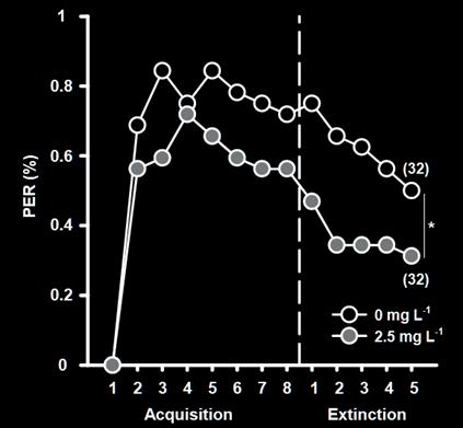
Balbuena et al. (2015) further demonstrated that glyphosate disrupts honeybee navigation, causing longer return times and increased orientation errors after exposure. Such cognitive deficits could reduce a bee’s willingness or ability to revisit treated flowers. Moreover, glyphosate’s effects extend beyond behaviour: Motta, Raymann, and Moran (2018) found that glyphosate perturbs the gut microbiota of honeybees, significantly reducing beneficial bacteria like Snodgrassella, which compromises immune function and nutrient absorption. These physiological stresses may diminish overall colony foraging vigour, indirectly lowering flower visitation rates.

Alteration of floral cues and rewards

Glyphosate may also indirectly deter pollinators by degrading floral rewards. Russo et al. (2023) reported that herbicide treatments reduce the amino acid content of pollen, and bees preferentially visit flowers offering higher nutritional quality. Fleury et al. (2020) similarly showed that glyphosate-based herbicides diminish nectar sugar concentration and alter volatile profiles, leading to lower pollinator visitation in field trials. In this study, bees may have detected these subtle quality changes and shifted foraging to untreated plots with richer rewards. Over time, such preferences could translate to decreased pollination in sprayed canola fields, with potential yield implications.

AI model performance

This study also evaluated AI-assisted monitoring via three YOLO-based model iterations. Model 1

exhibited high sensitivity but very low specificity, over-counting bees by misclassifying moving foliage or shadows as pollinator landings. This overfitting to non-bee features reflects training on a small, nonrepresentative dataset, a common pitfall in ecological deep learning applications (Bhuiyan et al., 2022). Model 2 addressed false positives by raising detection thresholds, achieving high precision but at the expense of low recall, it missed many actual bee visits. This sensitivity–specificity trade-off is well recognized in machine learning: improving one often degrades the other (Powers, 2011). Model 3 struck a better balance, detecting roughly 20–40% of true visits while keeping false alarms low; however, it still fell far short of the >90% accuracy reported in large-scale insect detection studies (Bjerge et al., 2023). Bjerge et al. built their system on nearly 30,000 annotated insect instances, illustrating that dataset scale and diversity are critical for robust performance. This study, with its smaller data-set, had a lot more variability in what could be defined as a bee visitation. Furthermore, the “black box” nature of deep learning hinders trust in AI outputs. Petsiuk et al. (2020) highlight the importance of explainable AI methods, such as saliency maps, to uncover the specific image regions influencing object detection decisions. Incorporating such visualization techniques could clarify whether our models accurately focus on bees rather than background distractions, thus guiding targeted improvements. As AI technologies become more prevalent in ecological research, integrating these explainability tools will be crucial to validate and refine automated monitoring before their widespread adoption. However, implementing these advanced explainability methods was beyond the scope of the current study, primarily due to constraints in time, resources, and technical expertise.

Multiple stressors and pollinator health

Glyphosate is only one of many stressors affecting bee populations. Goulson et al. (2015) synthesized evidence that pesticides, pathogens, and habitat loss act synergistically to drive declines in pollinator health. Other research has shown that exposure to multiple agrochemicals, such as insecticides, fungicides, and herbicides, can have additive or interactive sub-lethal effects on bee cognition and survival (Mengoni Goñalons & Farina, 2018). In realworld agricultural settings, bees often face these stressors simultaneously, which may amplify the behavioural and physiological disruptions observed in controlled studies. While this study isolates glyphosate to focus on its specific effects, future research should examine such multi-stressor interactions to better assess the full scope of risks facing pollinators in modern farming systems.

Study Limitations

Several constraints temper the conclusions. First, data were limited to two full days before sheep grazing halted the experiment, precluding statistical tests and replication. Weather variation between those days (sunny vs. cloudy) acted as a confounder, making it impossible to disentangle treatment effects from environmental noise. Floral density differed slightly among plots, introducing additional bias. Second, our AI models, while promising, underperformed due to limited training data and lack of explainable outputs, emphasizing that automated monitoring must be rigorously validated against human counts. Third, observations were confined to midday periods; bee foraging can vary diurnally, so our snapshots may not represent full-day patterns. These limitations mean our findings are exploratory, pointing to trends that warrant confirmation under more robust conditions.

Future directions

To build on these preliminary insights the following enhancements in a replicated study are recommended.

Experimental Controls and Replication

Establish multiple pairs of glyphosate-treated and control plots, ensuring uniform planting and bloom phenology. Use fencing or net enclosures to exclude livestock and minimize disturbances (Vicens & Bosch, 2000)

Extended Sampling

Collect data across a broader range of days, weather conditions, and times of day to achieve sufficient statistical power. Implement mixed-effects models to separate treatment effects from environmental variability

Expanded AI Training and Explainability

Annotate a significantly larger dataset (e.g., tens of thousands of bee instances) under diverse lighting and backgrounds. Explore advanced detection architectures (e.g., transformer-based models) and integrate saliency mapping or Grad-CAM to validate model focus (Petsiuk et al., 2021)

Multi-Stressors Assessment

Incorporate additional agrochemical exposures (e.g., insecticides, fungicides) in factorial designs to examine combined effects on bee cognition and foraging (Goulson et al., 2015)

By implementing these improvements, future research can more conclusively determine glyphosate’s impact on bee visitation and refine AI-assisted monitoring protocols, contributing to sustainable canola

production that safeguards both crop yields and bee health.

Conclusion

This study aimed to explore whether glyphosate herbicide applications affect pollinator visitation to Round-Up Ready Tru-Flex canola and assess if AIassisted monitoring could reliably track these effects. Despite methodological limitations, notably the unintended sheep intrusion and resulting data scarcity, preliminary insights were achieved.

Initial observations revealed reduced bee visitation to glyphosate-treated plots under favourable, sunny conditions, aligning with existing research indicating sub-lethal herbicide impacts on bee cognition (Balbuena et al., 2015; Farina et al., 2019) , physiology (Motta et al., 2018; Tan et al., 2022), and floral resource attractiveness (Russo et al., 2023) However, this trend was confounded by environmental variables, primarily weather, highlighting the complexity of attributing visitation differences solely to herbicide application.

The AI component, while promising, highlighted significant challenges: early models either over- or under-counted bees, while the final iteration provided improved but still limited accuracy. Key limitations included small training datasets, the models’ inherent "black box" nature, and insufficient data diversity, issues underscored by existing AI-pollinator research (Bjerge et al., 2023; Petsiuk et al., 2021)

Future studies should incorporate greater replication, enhanced experimental control (e.g., livestock exclusion, uniform floral density), expanded AI training datasets, and explainability techniques. Such refinements will clarify glyphosate’s ecological effects and enhance AI reliability, ultimately supporting sustainable canola production practices that balance herbicide use with pollinator health.

Acknowledgements

This research has been made possible by the College, Mrs Kathy Haigh and Dr Matthew Hill. Throughout this project, they have provided invaluable advice and guidance into my report.

References

Australian Agriculture: Broadacre Crops, 2023-24 financial year | Australian Bureau of Statistics. (2025, May 29).

https://www.abs.gov.au/statistics/industry/agriculture/austr alian-agriculture-broadacre-crops/latest-release

Balbuena, M. S., Tison, L., Hahn, M.-L., Greggers, U., Menzel, R., & Farina, W. M. (2015). Effects of sublethal doses of glyphosate on honeybee navigation. Journal of Experimental Biology, 218(17), 2799–2805. https://doi.org/10.1242/jeb.117291

Bhuiyan, T., Carney, R. M., & Chellappan, S. (2022). Artificial intelligence versus natural selection: Using computer vision techniques to classify bees and bee mimics. iScience, 25(9), 104924. https://doi.org/10.1016/j.isci.2022.104924

Bjerge, K., Alison, J., Dyrmann, M., Frigaard, C. E., Mann, H. M. R., & Høye, T. T. (2023). Accurate detection and identification of insects from camera trap images with deep learning. PLOS Sustainability and Transformation, 2(3), e0000051. https://doi.org/10.1371/journal.pstr.0000051

Catarino, R., Bretagnolle, V., Perrot, T., Vialloux, F., & Gaba, S. (2019). Bee pollination outperforms pesticides for oilseed crop production and profitability. Proceedings of the Royal Society B: Biological Sciences, 286(1912), 20191550. https://doi.org/10.1098/rspb.2019.1550

Farina, W. M., Balbuena, M. S., Herbert, L. T., Mengoni Goñalons, C., & Vázquez, D. E. (2019). Effects of the Herbicide Glyphosate on Honey Bee Sensory and Cognitive Abilities: Individual Impairments with Implications for the Hive. Insects, 10(10), Article 10. https://doi.org/10.3390/insects10100354

Goulson, D., Nicholls, E., Botías, C., & Rotheray, E. L. (2015). Bee declines driven by combined stress from parasites, pesticides, and lack of flowers. Science, 347(6229), 1255957. https://doi.org/10.1126/science.1255957

Karbassioon, A., Yearlsey, J., Dirilgen, T., Hodge, S., Stout, J. C., & Stanley, D. A. (2023). Responses in honeybee and bumblebee activity to changes in weather conditions. Oecologia, 201(3), 689–701. https://doi.org/10.1007/s00442-023-05332-x

Kongsilp, P., Taetragool, U., & Duangphakdee, O. (2024). Individual honey bee tracking in a beehive environment using deep learning and Kalman filter. Scientific Reports, 14(1), 1061. https://doi.org/10.1038/s41598-023-44718-y

Megoni Goñalons, C., & Farina, W. M. (2018). Impaired associative learning after chronic exposure to pesticides in young adult honey bees. Journal of Experimental Biology, 221(7), jeb176644. https://doi.org/10.1242/jeb.176644

Motta, E. V. S., Raymann, K., & Moran, N. A. (2018). Glyphosate perturbs the gut microbiota of honey bees. Proceedings of the National Academy of Sciences, 115(41), 10305–10310. https://doi.org/10.1073/pnas.1803880115

Petsiuk, V., Jain, R., Manjunatha, V., Morariu, V. I., Mehra, A., Ordonez, V., & Saenko, K. (2021). Black-box Explanation of Object Detectors via Saliency Maps (No. arXiv:2006.03204). arXiv. https://doi.org/10.48550/arXiv.2006.03204

Pollination of Crops in Australia and New Zealand. (2012). AgriFutures Australia https://agrifutures.com.au/product/pollination-of-crops-inaustralia-and-new-zealand/

Powers, D. M. (2011). Evaluation: From Precision, Recall and F-measure to ROC, Informedness, Markedness and Correlation. http://hdl.handle.net/2328/27165

Russo, L., Ruedenauer, F., Gronert, A., Vreken, I. V. de, Vanderplanck, M., Michez, D., Klein, A., Leonhardt, S., & Stout, J. C. (2023). Fertilizer and herbicide alter nectar and pollen quality with consequences for pollinator floral choices. PeerJ, 11, e15452. https://doi.org/10.7717/peerj.15452

Spiesman, B. J., Gratton, C., Hatfield, R. G., Hsu, W. H., Jepsen, S., McCornack, B., Patel, K., & Wang, G. (2021). Assessing the potential for deep learning and computer vision to identify bumble bee species from images. Scientific Reports, 11(1), 7580. https://doi.org/10.1038/s41598-02187210-1

Tan, S., Li, G., Liu, Z., Wang, H., Guo, X., & Xu, B. (2022). Effects of glyphosate exposure on honeybees. Environmental Toxicology and Pharmacology, 90, 103792. https://doi.org/10.1016/j.etap.2021.103792

The Influence of Time of Day on the Foraging Behavior of the Honeybee, Apis mellifera. (1989). https://doi.org/10.1177/074873048900400301

Vicens, N., & Bosch, J. (2000). Weather-Dependent Pollinator Activity in an Apple Orchard, with Special Reference to Osmia cornuta and Apis mellifera (Hymenoptera: Megachilidae and Apidae). Environmental Entomology, 29(3), 413–420. https://doi.org/10.1603/0046225X-29.3.413

Geographic Variation in Eastern Brown Snakes (Pseudonaja Textilis) venom composition: An

analysis of current research

Bowen Doak

Barker College

The Eastern Brown Snake (Pseudonaja textilis) is Australia's second most venomous and a medically significant reptile due to its distribution across diverse geographic regions from Queensland to South Australia, extending into the Northern Territory and Papua New Guinea. This analysis investigates the current state of research regarding geographic variation in Eastern Brown Snake venom composition and yield. Through systematic review of available literature, this study examines whether venom characteristics vary significantly between populations from different locations, potentially influenced by environmental factors such as temperature, prey availability, and local selective pressures. The research reveals limited but compelling evidence for geographic variation in venom yield and composition, with Queensland populations producing significantly higher venom yields compared to South Australian counterparts. However, substantial gaps remain in our understanding of the biochemical basis for these differences and their ecological significance. This analysis highlights the need for comprehensive, standardized studies of venom variation across the species' range to better inform antivenom development and snakebite treatment protocols.

Literature Review

Snake venoms represent complex biological cocktails that have evolved over millions of years as sophisticated tools for prey capture and defence. These venoms are not static entities but dynamic systems that can vary significantly both within and between species populations. Understanding this variation is crucial for multiple reasons: improving antivenom efficacy, predicting clinical outcomes of envenomation, and advancing our knowledge of evolutionary biology and toxicology.

The Eastern Brown Snake (Pseudonaja textilis) stands as one of Australia's most formidable venomous species, ranking second in global toxicity rankings and responsible for approximately 68% of snakebites and 41% of death caused by snakebites in Australia (This Snake Is a PROBLEM, 2025). This species exhibits remarkable geographic distribution, spanning the eastern coastline of Australia from Queensland to South Australia, with populations extending into the Northern Territory near Darwin and reaching into Papua New Guinea (Figure 1). Such extensive distribution across varied climatic zones and ecosystems provides an ideal model system for investigating geographic variation in venom characteristics. Venom characteristics include the biochemical composition, the potency and volume of venom used. These characteristics allow researchers

to create individualised responses as well as to highlight similarities and variances across species.

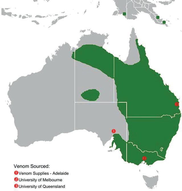
Figure 1: Eastern Snake Distribution and research locations across Australia and Papua New Guinea

Recent research on other venomous species has demonstrated significant geographic variation in venom composition. Studies on American rattlesnakes have revealed latitudinal gradients in venom components, particularly snake venom metalloproteinases (SVMPs) and mycotoxins, correlating with distance from the equator (Mackessy, 2010). Similarly, research on Australian funnel-web

spiders has led to the discovery of new species variants, such as the "Newcastle Big Boy," highlighting the importance of geographic considerations in venomous animal research. From the research the information was generally gathered either from a clinical review of veterinary cases of envenomation or from a study of a specific factor of the venom within one area.

Specific Predictions

This variation is predicted to manifest across three primary dimensions. First, venom yield differences are expected between populations, with those inhabiting prey-rich environments predicted to produce higher venom yields per extraction compared to populations in resource-limited habitats. This prediction is based on the rationale that metabolic investment in venom production should correlate with prey availability and predation pressure. The measurable outcome would be significant differences in milligrams of venom per gram of body weight between geographic populations.

Second, biochemical composition is expected to vary systematically between populations, specifically in the relative concentrations of major toxin classes including phospholipase A₂, metalloproteinases, hyaluronidases, coagulants, and neurotoxins. The underlying rationale is that local prey assemblages and their physiological vulnerabilities should drive selection for optimal toxin cocktails tailored to regional prey species. This would manifest as statistically significant differences in toxin class ratios as determined by proteomic analysis and enzymatic assays.

Third, biological activity profiles are predicted to demonstrate variable functional potency, with venom from different populations showing distinct performance against standardized bioassays that reflect adaptation to local prey species. The rationale for this prediction is that functional optimization of venom for local prey should result in measurable differences in lethality, coagulation effects, and tissue damage rates. The expected measurable outcome would be significant variation in LD₅₀ values, coagulation times, and haemolytic activity between geographic populations.

Scientific Research Question

This study addresses the research question: How does Eastern Brown Snake venom vary by geographic location based on current available information?

Scientific Hypothesis

Based on established ecological theory regarding local adaptation and documented patterns of intraspecific venom variation observed in other venomous species (including Bothrops pit vipers, Naja cobras, and Crotalus rattlesnakes), it is hypothesized that Eastern Brown Snake (Pseudonaja textilis) populations will exhibit significant geographic variation in venom characteristics across their continental Australian range.

Underlying Theoretical Framework

This hypothesis is based on the Geographic Mosaic Theory of Coevolution and the Theory of Local Adaptation, which propose that geographically isolated populations diverge in traits in response to local selective pressures. The venom system, as a critical adaptive interface between predator and prey, is especially prone to geographic variation driven by factors such as local prey composition and abundance, climatic influences on venom stability and delivery, population genetic structure and gene flow, and historical biogeographic processes.

Testable Implications

If supported, this hypothesis would indicate that Eastern Brown Snake venom is a geographically structured adaptive trait. Such a finding would have important implications for several areas, including the development of more effective antivenoms and refinement of clinical treatment protocols, deeper insights into the evolutionary dynamics of venom systems, improved understanding of the conservation genetics of venomous species, and a more nuanced view of biogeographic patterns of predator-prey coevolution across Australia.

Methodology

Search Strategy

A systematic literature search was conducted using Google Scholar as the primary database. Then using the criteria outlines below (Table 1) the search results were screened and selected to those that were most relevant to the study.

Table 1: Literature search terms and selection inclusions and exclusions

Criteria information

Search terms

Systematic literature search conducted on Google Scholar data base primarily whilst emphasising the following terms:

“Eastern brown snake venom”, “Eastern Brown snake venom comparison”, “Eastern Brown snakes NSW", “Eastern Brown snakes PNG”, “Pseudonaja Textilis venom components”, “Eastern Brown snake

venomics”, “Veterinary reports of Eastern Brown snake bites”, “SnakeMap project”

Inclusion Contained quantitative or qualitative data on P. textilis venom properties.

Contained the geographic origin of venom source.

Medical data both veterinary and clinical with location specification

Comparative of P. textilis venom with other snakes within or other species

Exclusion Did not contain a clear geographical location to the obtaining of the venom used.

Used pooled venom from multiple snakes in a group without having singular tests.

Theoretical or review paper lacking original data.

Only includes antivenom development without including venom specifics of the characterisation.

Data Extraction and Analysis

Data extraction focused on several key parameters, including the geographic origin of venom samples, venom yield measurements, biochemical composition data, and biological activity profiles. Additional attention was given to sample sizes and collection methods, as well as the degree of standardization in collection protocols, to ensure consistency and reliability across studies.

Results

Literature Search Outcomes

The systematic search yielded nine primary studies meeting inclusion criteria, spanning research from 1998 to current day. These studies varied significantly in scope, methodology, and geographic coverage, with most samples originating from South Australia and Queensland populations.

Summary

Mirtschin PJ, Shine R, Nais TJ, Dunstan NL, Hough BJ, Mirtschin M

Useful baseline data, though focuses more on size dimorphism than venom composition

Queensland animals produced 3x more venom than South Australian specimens (11 vs 3 mg average). Percent solids were inversely related (20% vs 22%) respectively (F1;48 1⁄4 15:49; P , 0.001).

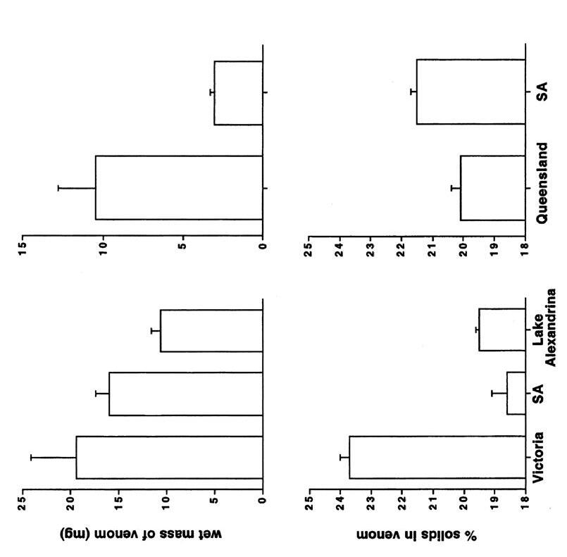
Influence on venom yield in Australian tiger snakes and brown snakes. 7 May 2002 53 eastern browns over 4 years; venom from Venom Supplies Pty Ltd, Tanunda. This venom was labelled as Queensland or South Australia. Venom yield analysis (dry mass quantities)

1

Cipriani V, Debono J, Goldenberg J, Jackson T, Arbuckle K, et al.

Provides broader baseline for P. textilis venom within genus context

Genuslevel venom similarities identified. Juvenile P. textilis venom lacks Factor Xa, while adults contain large quantities

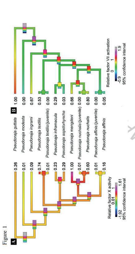
Comparative venom composition across Pseudonaja species (P. affinis, P. aspidorhyncha, P. gutta)

Venom from Venom Supplies Pty Ltd and University of Queensland Venom Evolutionary Lab

Correlation between ontogenetic dietary shifts and venom variation in Australian brown snakes (Pseudonaja). Comparative Biochemistry and Physiology Part C: Toxicology & Pharmacology, 197, 5360. 2017

2

Limited scopesingle protein analysis

Structural similarities to aprotinin identified

Crystalline structure of textilinin1 protein

Cloned structure from BresaGen, Adelaide

Crystallization and preliminary Xray analysis of a Kunitztype inhibitor, textilinin1 from Pseudonaja textilis textilis Acta

Crystallographica Volume 62 part 7, pages 642645 1 July 2006

Millers EK, Masci PP, Lavin MF, de Jersey J, Guddat LW 4

3

Rao VS, Swarup S, Kini RM

Specific focus on coagulation mechanisms

Structural similarity to mammalian coagulation factor V

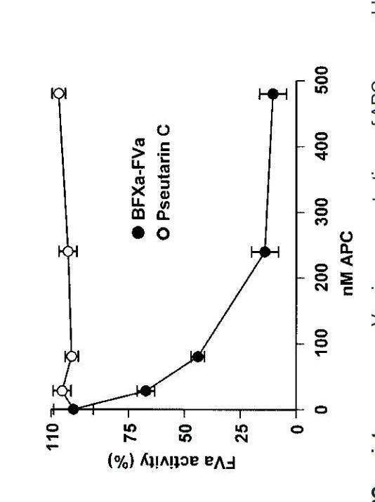
Procoagulating features, specifically pseutarin C structure

Venom Supplies Australia

The nonenzymatic subunit of pseutarin C, a prothrombin activator from eastern brown snake (Pseudonaja textilis) venom Blood, August 15, 2003, in volume 102, issue 4, pages 13471354

Xu, H., ElAsal, S., Zakri, H., Mutlaq, R., Krikke, N., Casewell, N., Slagboom, J. and Kool J.

Methodological value for future studies

Comparison of two venom preparation techniques for analysis

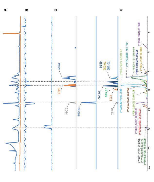
Analytical methodology comparison

University of Melbourne (multiple organisms including P. textilis)

Aligning PostColumn ESIMS, MALDIMS, and Coagulation Bioassay Data of … Pseudonaja textillis Venoms Chromatographic ally …” Toxins (MDPI) 2024

5

Smith, C.F., Nikolakis, Z.L., Ivey, K. et al.

Excellent model for geographic venom variation studies (different species)

Linear relationship: mycotoxins increase toward equator, SVMPs increase away from equator

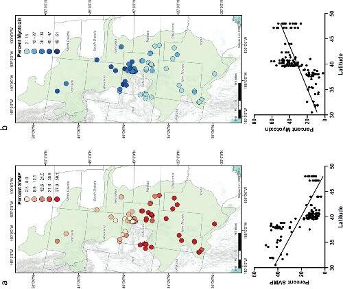
Central America (multiple locations) SVMP and mycotoxin percentages in rattlesnake venom

Snakes on a plain: biotic and abiotic factors determine venom compositional variation in a wideranging generalist rattlesnake. BMC Biol 21, 136 2023

6

Masci PP, Mirtschin PJ, Nias TN, Turnbull RK, Kuchel TR, et al.

Limited to two locations; focuses on quantity rather than composition

Higher venom yields than previously reported across all species

Higher venom yields than previously reported across all species

Venom yield comparison across Pseudonaja genus

40 specimens from Adelaide, SA; 14 from Gold Coast, QLD (Venom Supplies Pty Ltd)

7 Brown Snakes (Pseudonaja Genus): Venom Yields, Prothrombin Activator Neutralization and Implications for Antivenom Anaesthesia and Intensive Care in 1998

Heller J, Bosward KL, Hodgson JL, Cole FL, Reid SW, Hodgson DR, and Mellor DJ

Qualitative data only; limited numerical value

Statistical analysis of venom effects on domestic animals

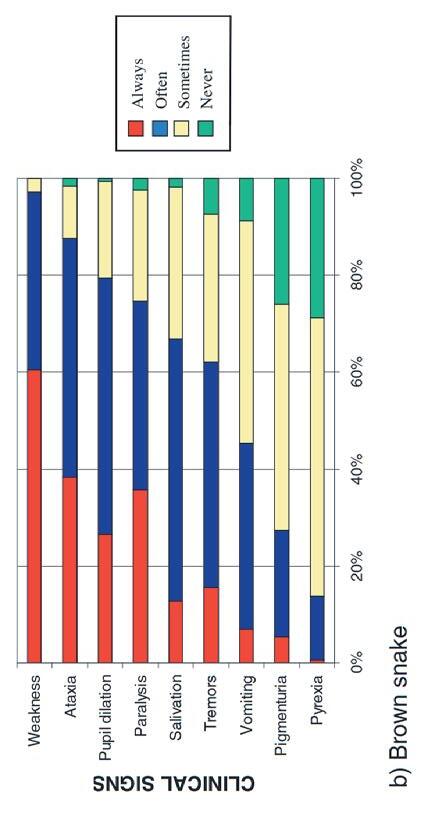
Clinical effects of brown snake envenomation

Snake envenomation in dogs in New South Wales Australian Veterinary Journal in 2005 (volume 83, issue 5, pages 286292) NSW veterinary clinics (questionnairebased)

8

2 Mirtschin PJ, Masci P, Paton DC, Kuchel T

Eastern brown snakes have 10 times more envenomation cases than other species in Australia

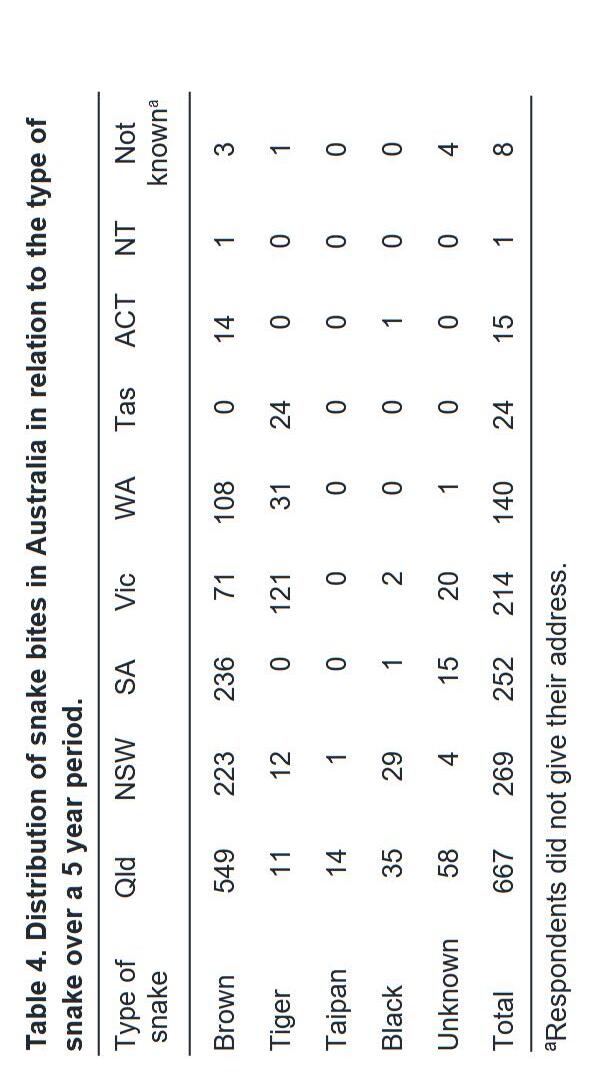
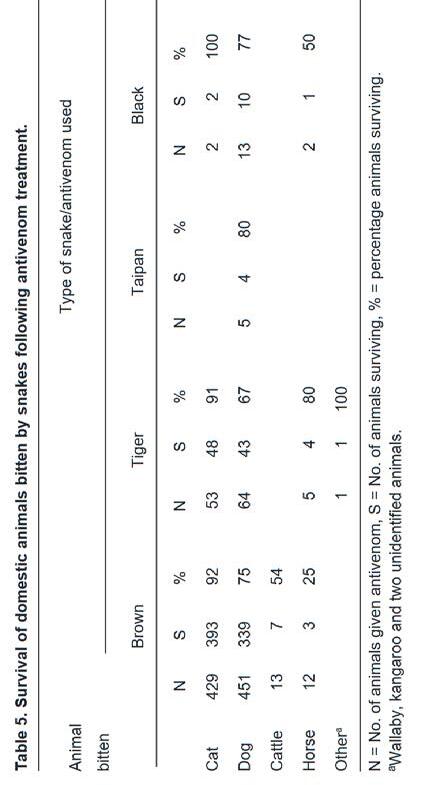
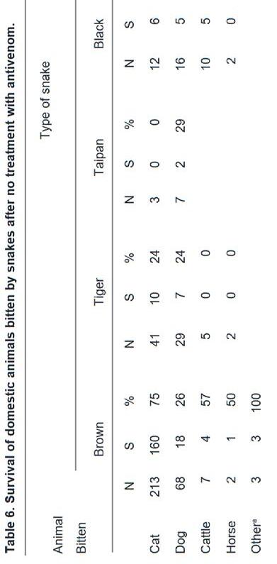
Lethality, attack likelihood, and geographic distribution

Snake bites recorded by veterinary practices in Australia Australian Veterinary Journal in 1998 (volume 76, pages 1958) 10% of Australian veterinary clinics (questionnaire)

Geographic Distribution of Research

Research coverage shows significant bias toward easily accessible populations:

• South Australia: 3 studies (primarily Adelaide region)

• Queensland: 1 studies (Gold Coast and Brisbane regions)

• New South Wales: 2 studies (primarily veterinary reports)

• Northern Territory: 0 specific studies

• Papua New Guinea: 0 specific studies

• South Australia and Queensland: 2 studies

• East coast Australia: 1 study

Venom Yield Variation

The most robust evidence for geographic variation comes from yield studies comparing Queensland and South Australian populations.

Key Finding: Mirtschin et al. (2002) demonstrated that Queensland Eastern Brown Snakes produced approximately three times more venom than South Australian conspecifics (11 mg vs. 3 mg dry weight, F₁,₄₈ = 35.76, P < 0.0001).

However, this difference correlates with known size dimorphism between populations, with Queensland snakes significantly larger than South Australian specimens. The biological significance of this yield difference remains unclear when controlling for body size. Interestingly, percent solids showed an inverse relationship, with South Australian snakes producing more concentrated venom (22% vs. 20% solids, F₁,₄₈ = 15.49, P < 0.001).

Biochemical Composition Studies

Limited data exists on geographic variation in venom biochemistry: Factor Xa Activity: Cipriani et al. (2017) noted developmental differences in Factor Xa presence, with juvenile P. textilis lacking this coagulation factor while adults showed substantial quantities. However, geographic variation in Factor Xa activity was not systematically examined.

Prothrombin Activator Components: Studies of pseutarin C, a major prothrombin activator in P. textilis venom, have been conducted primarily on South Australian samples, limiting geographic comparisons.

Clinical and Veterinary Evidence

Veterinary studies from New South Wales provide indirect evidence of venom variation through differential clinical presentations but lack the quantitative rigor necessary for definitive conclusions about geographic variation. It only showed an overall

trend of the state which would be extremely beneficial if the exact same study was conducted within the other states where this snake is present.

Envenomation Patterns

NSW veterinary data suggests variation in clinical symptom presentation, but multiple confounding factors (victim size, bite location, venom delivery efficiency and seasonality) preclude clear attribution to geographic venom differences. It is a useful basis to design a hypothesis but the lack of available comparative information between cases means that there is limited uses within this report.

Discussion

Evidence for Geographic Variation

This analysis reveals limited but compelling evidence for geographic variation in Eastern Brown Snake venom characteristics across the nine studies. The most robust findings relate to venom yield differences between Queensland and South Australian populations, though this may primarily reflect body size dimorphism rather than intrinsic venom gland differences.

The observed inverse relationship between venom quantity and concentration suggests potential adaptive trade-offs. South Australian populations may compensate for smaller venom yields through increased toxin concentration, potentially reflecting adaptation to different prey communities or environmental constraints. Whereas in Queensland the snakes have had a large increase in venom quantity as well as size of the snakes which could be reflective of availability of smaller scale prey items or due to the reduction of natural predators.

Ecological Implications

Several ecological factors may drive venom variation across the P. textilis range For example, the species' range spans significant climatic variation, from tropical Queensland to temperate South Australia. Temperature differences may influence venom protein stability, prey activity patterns, and metabolic costs of venom production.

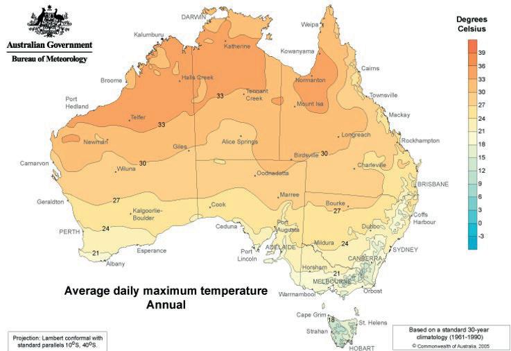
Figure 2: Topographical map of Australia with temperature comparison from 1961-1990 (Source: Australia Daily Annual Maximum Temperature Averages Map, 2006.)

This map shows a trend that is expected that the closer to the equator the warmer the temperature. This is beneficial for the study of snakes as the warm temperatures allow for more energy due to the coldblooded nature of reptiles. Therefore, the snake in Queensland have more time and energy to invest in hunting and other activities.

Furthermore, each of the different regions host distinct prey assemblages. Northern populations may encounter different small mammal communities, potentially selecting for different toxin profiles optimized for local prey such as prioritising a paralysis agent to allow for the smaller animal to be eaten hole. Whereas within South Australia, the amount of prey is smaller and this means that the snake needs to be more affluent at hunting a larger mixture of available animals, as well as being able to commit minimal energy into securing a kill. Lastly, the Habitat Differences, such as coastal woodlands to semi-arid scrublands habitat variation would further influence prey specific to that area, as well encounter rates and thus cause a divergence for the optimal venom strategies for the snakes.

Comparative Context

The limited evidence for geographic variation in P. textilis contrasts with more dramatic patterns observed in other venomous species. American rattlesnakes show clear latitudinal gradients in SVMP and mycotoxin composition (Mackessy, 2010), while some Australian elapids exhibit pronounced regional variation in neurotoxin profiles.

This difference may reflect several underlying factors, including the relatively recent evolutionary radiation of Pseudonaja textilis across its range and strong gene flow between populations, which may maintain venom homogeneity. Additionally, the species’

generalist prey preferences could reduce the selective pressure for location-specific venom adaptations. Finally, the apparent uniformity may also be influenced by the limited resolution and scope of current research studies. Thus, we must consider external cases where a more in-depth study was performed as it could also reveal a possible pattern within the venom characteristics.

Clinical Implications

Understanding geographic venom variation has direct clinical relevance.

Antivenom Efficacy

If significant biochemical variation exists, antivenoms developed using venom from one region may show reduced efficacy against bites from other regions. It might also create excess immunoglobulin from the antivenom which could mistake necessary cells for the venom and cause a larger reaction.

Treatment Protocols:

Regional variation in venom composition could necessitate location-specific treatment approaches or modified antivenom dosing regimens. The variation would also prove that specific creation of antivenom must be done with selective care as the surrogate for the venom might not have a resistance to the different forms of the venom.

Risk Assessment:

Areas with populations producing higher venom yields or more potent compositions may require enhanced preparedness and rapid response capabilities. Furthermore, by having a more specific antidote you are reducing the foreign substances that could be considered as an allergen to a subject therefore you would reduce the chances of having a allergic reaction to the treatment.

Limitations

Several methodological limitations constrain this analysis. These include the limited availability of standardized, location-specific venom data and a reliance on samples predominantly sourced from commercial suppliers such as Venom Supplies Pty Ltd. Additionally, the lack of consistent biochemical analysis methods across studies hampers direct comparisons, while small sample sizes for specific geographic locations further limit the robustness and generalizability of the findings. A further limitation is that some papers are confidential as they relate patient health.

Research Gaps and Future Directions

This analysis reveals substantial gaps in current knowledge:

Geographic Coverage

Extensive regions remain unstudied, particularly Northern Territory and Papua New Guinea populations. These regions if studied could reveal a greater degree of venom variation than predicted due to isolation and distinct environmental conditions.

This means that these areas, specifically PNG, could show an extreme result of divergent evolution due to the land isolation from Australian brown snakes and how their environment is significantly different than those seen within the Australian population.

Biochemical Resolution

Most studies focus on crude venom properties rather than detailed biochemical profiling. Advanced proteomics and transcriptomics approaches could reveal subtle but clinically significant composition differences.

Standardization

Lack of standardized collection, storage, and analysis protocols across studies limits comparative analysis. Future research requires coordinated, standardized approaches so that studies can be compared internally for a pattern to emerge.

Sample Sizes

Many studies rely on small sample sizes inadequate for detecting moderate effect sizes. Larger, population-level sampling is essential. Furthermore, the larger sample sizes were not clearly defined, often being a pooled source of venom with no point of origin.

Temporal Variation

No studies address seasonal or multi-year variation in venom characteristics, which could confound geographic comparisons. There was one study into the effect of captivity on the venom, but it was concluded that there was no effect on the venom.

Conclusion

This analysis provides the first systematic evaluation of geographic variation in Eastern Brown Snake venom characteristics. While evidence for variation exists, particularly in venom yield and concentration, current research remains insufficient to draw definitive conclusions about the extent and clinical significance of geographic differences.

Key Findings:

1. Queensland populations produce significantly higher venom yields than South Australian populations.

2. South Australian populations produce more concentrated venom.

3. These differences may primarily reflect body size dimorphism rather than adaptive venom variation.

4. Substantial research gaps exist, particularly for northern and eastern populations.

Research Priorities:

1. Comprehensive sampling across the entire species range, particularly understudied regions.

2. Standardized biochemical profiling using modern analytical techniques.

3. Integration of ecological, genetic, and toxicological approaches.

4. Clinical correlation studies examining regional variation in envenomation outcomes.

Understanding geographic variation in P. textilis venom has implications extending beyond academic interest. As Australia's most medically significant venomous snake, comprehensive knowledge of venom variation could improve clinical outcomes, optimize antivenom development, and enhance our understanding of venom evolution. The limited current evidence suggests variation exists but remains insufficiently characterized to guide clinical practice or inform evolutionary hypotheses.

Future research must address these knowledge gaps through coordinated, large-scale studies employing standardized methodologies across the species' range. Only through such comprehensive investigation can we fully understand the extent and significance of geographic variation in Eastern Brown Snake venom.

Acknowledgements

I would like to thank the tireless work of Professor Bryan Fry and Peter Mirtschin who have published countless papers.

Professor Fry has a double degree in Molecular Biology and Scientific Philosophy together with a PhD on the toxic natriuretic peptides of the inland taipan. He has conducted field research in over 40 countries and appeared in over 100 documentaries. He has been inducted into the elite adventurer society The Explorers Club – having broken 23 bones in the field, including his back. He has had 400 stitches, three concussions, a near fatal scorpion sting in the

Amazon, a nasty centipede sting in Costa Rica and a stone fish sting. He has devoted his life (and body) to the study of venom.

Peter Mirtschin is a renowned Australian toxinologist, herpetologist, and conservationist who has made significant contributions to snake venom research and Australian herpetology over several decades. Peter founded Venom Supplies, which supplies both Australian and exotic snake venoms for research, antivenom and therapeutic applications. He has published around 85 scientific papers on venom research, snake ecology, conservation, and snake behaviour, as well as several books on Australian dangerous snakes. Peter has featured in several television documentaries, being an ardent resultsdriven conservationist.

References

Australia Daily Annual Maximum Temperature Averages Map. (n.d.). Retrieved June 24, 2025, from https://eldoradoweather.com/forecast/australia/australiadaily-maximum-temperatures.html

Cipriani, V., Debono, J., Goldenberg, J., Jackson, T. N. W., Arbuckle, K., Dobson, J., Koludarov, I., Li, B., Hay, C., Dunstan, N., Allen, L., Hendrikx, I., Kwok, H. F., & Fry, B. G. (2017). Correlation between ontogenetic dietary shifts and venom variation in Australian brown snakes (Pseudonaja). Comparative Biochemistry and Physiology Part C: Toxicology & Pharmacology, 197, 53–60. https://doi.org/10.1016/j.cbpc.2017.04.007

Fry, B. G., Scheib, H., Van Der Weerd, L., Young, B., McNaughtan, J., Ramjan, S. F. R., Vidal, N., Poelmann, R. E., & Norman, J. A. (2008). Evolution of an Arsenal. Molecular & Cellular Proteomics, 7(2), 215–246. https://doi.org/10.1074/mcp.M700094-MCP200

Fry, B. G., W�ster, W., Kini, R. M., Brusic, V., Khan, A., Venkataraman, D., & Rooney, A. P. (2003). Molecular Evolution and Phylogeny of Elapid Snake Venom ThreeFinger Toxins. Journal of Molecular Evolution, 57(1), 110–129. https://doi.org/10.1007/s00239-003-2461-2

Heller, J., Bosward, K., Hodgson, J., Cole, F., Reid, S., Hodgson, D., & Mellor, D. (2005). Snake envenomation in dogs in New South Wales. Australian Veterinary Journal, 83(5), 286–292. https://doi.org/10.1111/j.17510813.2005.tb12743.x.

Mackessy, S. P. (2010). Evolutionary trends in venom composition in the Western Rattlesnakes (Crotalus viridis sensu lato): Toxicity vs. tenderizers. Toxicon, 55(8), 1463–1474. https://doi.org/10.1016/j.toxicon.2010.02.028

Millers, E.-K. I., Masci, P. P., Lavin, M. F., de Jersey, J., & Guddat, L. W. (2006). Crystallization and preliminary X-ray analysis of a Kunitz-type inhibitor, textilinin-1 from Pseudonaja textilis textilis. Acta Crystallographica Section F: Structural Biology and Crystallization Communications, 62(7), 642–645. https://doi.org/10.1107/S1744309106019099

Mirtschin, P. J., Shine, R., Nias, T. J., Dunstan, N. L., Hough, B. J., & Mirtschin, M. (2002). Influences on venom yield in Australian tigersnakes (Notechis scutatus) and

brownsnakes (Pseudonaja textilis: Elapidae, Serpentes). Toxicon, 40(11), 1581–1592. https://doi.org/10.1016/S0041-0101(02)00175-7.

Mirtschin, P., Masci, P., Paton, D., & Kuchel, T. (1998). Snake bites recorded by veterinary practices in Australia. Australian Veterinary Journal, 76(3), 195–198. https://doi.org/10.1111/j.1751-0813.1998.tb10128.x

Rao, V. S., Swarup, S., & Kini, R. M. (2003). The nonenzymatic subunit of pseutarin C, a prothrombin activator from eastern brown snake (Pseudonaja textilis) venom, shows structural similarity to mammalian coagulation factor V. Blood, 102(4), 1347–1354. https://doi.org/10.1182/blood-2002-12-3839

Smith, C. F., Nikolakis, Z. L., Ivey, K., Perry, B. W., Schield, D. R., Balchan, N. R., Parker, J., Hansen, K. C., Saviola, A. J., Castoe, T. A., & Mackessy, S. P. (2023). Snakes on a plain: Biotic and abiotic factors determine venom compositional variation in a wide-ranging generalist rattlesnake. BMC Biology, 21(1), 136. https://doi.org/10.1186/s12915-023-01626-x

Sutherland, S. K., & Tibballs, J. (2001). Australian animal toxins: The creatures, their toxins, and care of the poisoned patient (2nd ed). Oxford University Press.

This snake is a PROBLEM. (2025, June 6). [Video recording].

https://www.youtube.com/shorts/CgFfHhA8BAM

Xu, H., El-Asal, S., Zakri, H., Mutlaq, R., Krikke, N. T. B., Casewell, N. R., Slagboom, J., & Kool, J. (2024). Aligning Post-Column ESI-MS, MALDI-MS, and Coagulation Bioassay Data of Naja spp., Ophiophagus hannah, and Pseudonaja textillis Venoms Chromatographically to Assess MALDI-MS and ESI-MS Complementarity with Correlation of Bioactive Toxins to Mass Spectrometric Data. Toxins, 16(9), Article 9. https://doi.org/10.3390/toxins16090379

What role does ecological adaptation play in the development of tool-use behaviour in Choerodon wrasses?

Ally Habgood Barker College

This research investigates the role of ecological adaptation in developing tool use behaviour in Choerodon wrasses. Data was compiled from FishBase and Fishes of Australia by examining relevant literature to assess habitat, diet, and documented tool use cases. Findings indicate that ecological pressures, such as prey accessibility and environmental factors, shape behavioural adaptations leading to tool use. Phylogenetic perspectives highlight evolutionary transitions linked to foraging strategies. The study concludes that ecological factors significantly influence tool use behaviour, providing insights into marine species’ cognitive abilities and evolutionary trends.

Literature Review

The wrasse, a diverse family of reef-associated fish found throughout the Indo-Pacific region, includes several species noted for their complex behaviours and ecological specialisations. Of particular interest is the genus Choerodon, such as the Blackspot Tuskfish (Choerodon schoenleinii), which inhabit coral reef systems and have attracted scientific attention for their apparent use of tools. Tool use, once thought to be exclusive to higher vertebrates such as primates and certain birds, is now recognised across a broader spectrum of taxa, including fish. In this context, tool use refers to the manipulation of external objects to achieve a goal, such as using rocks or coral surfaces as anvils to break open hard-shelled prey. This behaviour not only challenges long-standing assumptions about animal cognition but also invites investigation into the ecological and evolutionary factors, such as habitat complexity and dietary needs, that may drive such behaviours in coral fish. These behaviours can be understood as examples of ecological adaptation, the process by which organisms develop traits or behaviours that enhance their survival and reproduction within specific environmental contexts. In the case of Choerodon, their tool use may represent an adaptive response to the demands of exploiting hard-shelled prey within the structurally complex reef environment.

Although tool use has traditionally been associated with higher vertebrates, emerging evidence reveals that this behaviour is more widespread in the animal kingdom, including among fish. Brown (Brown, 2015) documents tool use behaviour in Blackspot Tuskfish (Choerodon schoenleinii), which has been seen cracking molluscs against rocks, indicating a level of problem-solving and motor coordination. In a comparable case, archerfish employ direct water jets

to dislodge prey from overhanging vegetation, suggesting that diverse aquatic species may share convergent cognitive strategies for foraging. Similarly, Jaishankar (Jaishankar, 2024) reports that species such as Halichoeres and Thalassoma wrasses have been observed using hard surfaces, often referred to as anvils, to break open the protective shells of their prey, demonstrating deliberate object manipulation to access food. These findings challenge the notion that tool use is a rare evolutionary trait and highlight its potential ecological function in aquatic environments. Expanding on the cognitive aspects, Paśko (Paśko, 2010) presents evidence of memory-based tool use in six-bar wrasses, demonstrating that these fish can recall the location of suitable “anvils” to process prey, highlighting the role of spatial memory in foraging. Paśko also explores the impact of environmental enrichment, such as increased habitat complexity and access to diverse stimuli, on the cognitive performance of reef fish, suggesting that enriched environments promote behavioural flexibility and innovation. Further, Paśko’s, evolutionary review of reef-associated fish provides broader insights into species diversification and ecological interactions, emphasising how behavioural adaptations like tool use are shaped by phylogenetic history and ecological pressures. This integrative perspective strengthens the argument that tool use in wrasses is not merely incidental but may reflect deeper evolutionary and cognitive traits. Adam and Toledo (Adam & Toledo, 2025) propose a series of systematic experiments to further investigate tool use behaviours in wrasse, aiming to determine whether these behaviours are spontaneous, learned, or dependent on environmental context. Their proposed studies include controlled observations of wrasses interacting with objects in modified habitats, designed to assess problem-solving abilities and the consistency of tool use across individuals and conditions.

Floeter (Floeter, 2018) explores how ecological factors such as diet, body size, water column usage, and geographic range contribute to the evolutionary diversification of reef fish, including wrasses. Through comprehensive phylogenetic analyses, the study reveals multiple independent transitions to planktivory, the specialised feeding on plankton, across various lineages. These transitions suggest that shifts in dietary strategy can drive speciation, the evolution process by which new and distinct species emerge. Furthermore, variations in geographic range among reef fish populations point to vicariant processes, where physical or ecological barriers lead to genetic divergence and species isolation. By integrating both phylogenetic and functional ecological, Floeter’s work enhances the understanding of how community structures form within coral reef ecosystems. This perspective provides valuable context for examining the evolution of complex behaviours, such as tool use, in response to ecological pressures and adaptive challenges faced by species like Choerodon wrasses.

Jacobs and Osvath (Jacobs & Osvath, 2016) examine the cognitive processes that underpin tool use, emphasising key functions such as problem-solving, mental representation and foresight, traits once believed to be limited to higher mammals. Their work suggests that tool use requires not only physical ability but also the ability to anticipate outcomes and plan actions, accordingly, providing important insight into the cognitive sophistication of species like wrasses. Brown (Brown, 2015) also argues that the growing evidence of complex behaviours in fish, such as memory, learning and tool use, demands a reevaluation of how fish intelligence is perceived, particularly in the context of scientific research and commercial fisheries. This has important ethical implications, especially concerning welfare standards and the moral consideration of fish in experimental and industrial practices. Complementing these perspectives, Crain (Crain et al., 2013) advocates for the development of a universal, cross-species definition of tool use. They argue that a consistent framework is essential for comparative analysis, allowing researchers to better evaluate behavioural similarities and differences across taxa. Together, these studies support a growing recognition of fish as cognitively capable organisms, reinforcing the significance of studying tool use through both ecological and philosophical lenses.

Scientific Research Question

What role does ecological adaptation play in the development of tool use behaviour in Choerodon wrasses?

Scientific Hypothesis

Ecological adaptation significantly influences the development of tool use behaviour in Choerodon wrasses.

Methodology

Data was collected from two primary online databases, FishBase and Fishes of Australia, chosen for their scientific reliability, comprehensive coverage, and taxonomic accuracy. These databases were selected because they provided curated, speciesspecific information compiled by marine biologists, including geographic distribution, dietary habits, habitat preferences, and ecological roles of Choerodon species. Their accessibility and consistency across records allowed for the efficient extraction and comparison of environmental and biological data.

Peer-reviewed journal articles were selected through targeted searches in databases such as Google Scholar, Web of Science, and ScienceDirect. Search terms included combinations of “Choerodon,” “wrasse,” “tool use,” “foraging behaviour,” and “ecological adaptation,”. Articles were chosen if they met one or more of the following criteria:

1) If they were published in reputable, peerreviewed journals.

2) If they addressed the behavioural or ecological aspects of the Choerodon species.

3) If they specifically discussed evidence of tool use or analogous behaviours in wrasses or other reef fish. Preference was given to studies conducted in the Indo-Pacific region to ensure ecological relevance.

The data collection process involved accessing journal articles from freely available sources, and if articles were behind paywalls, then information from abstracts and summaries was used. Additionally, while both FishBase and Fishes of Australia provide extensive species records, potential discrepancies in update frequency and regional data granularity may have influenced the completeness of the data retrieved.

Results

Findings indicate a correlation between habitat variability and tool-use behaviour. Choerodon wrasses inhabiting diverse reef environments exhibit higher frequencies of tool use, particularly in prey manipulation strategies.

Table 1: Choerodon wrasses environment, diet and tool use behaviour

Fish Name Tool Use

Location

Blue tuskfish (Choerodon cyanodus) Yes Shallow reef Hard Shelled Prey Indopacific

Orange-dotted tuskfish (Choerodon anchorago) Yes Shallow reef Hard Shelled Prey Indian Ocean

Blackspot tuskfish (choerodon schoenleinii) Yes

Baldchin groper (choerodon rubescens) Yes

Shallow weed/sand Hard Shelled Prey Indopacific

Shallow coral Soft prey (Octopi, etc) +Sea Urchins Western Australia

Purple Tuskfish (Choerodon cephalotes) Yes Shallow coral Hard Shelled Prey Western Australia

Graphic Tuskfish (Choerodon graphicus) Yes

Shallow rocky reef Hard Shelled Prey Western Pacific

Azurio tuskfish (Choerodon azurio) Yes Deep rocky reef Soft prey (Shrimp, etc) +Sea Urchins Western Pacific

Swallowtail tuskfish (Choerodon cypselurus) Unknown Deep weed/sand Hard Shelled Prey Indo-west Pacific

Dark-spot tuskfish (Choerodon monostigma) Unknown Shallow weed/sand Hard Shelled Prey Western Pacific

Robust tuskfish (Choerodon robustus) Unknown Deep rocky reef Hard Shelled Prey Indopacific

Purple eyebrowed tuskfish (Choerodon zamboangae) Yes Deep weed/sand Hard Shelled Prey Indo-west Pacific

Orange-dotted tuskfish (Choerodon anchorago) Yes Shallow weed/sand Hard Shelled Prey +Sea Urchins Indo-west Pacific

Bluespotted tuskfish (Choerodon cauteroma) Yes Deep reef Hard Shelled Prey Western Australia

White-patch tuskfish (Choerodon oligacanthus) Unknown Shallow reef Hard Shelled Prey Western Pacific

Venus tuskfish (Choerodon venustus) Yes Deep weed/sand Hard Shelled Prey Eastern Australia

Harlequin tuskfish (Choerodon fasciatus) Unknown Shallow reef Hard Shelled Prey Indopacific

Redstripe tuskfish (Choerodon vitta) Unknown Shallow reef Hard Shelled Prey Western Pacific

Whitestripe tuskfish (Choerodon albofasciatus) Unknown Deep reef Hard Shelled Prey Western Australia

Gilded tuskfish (Choerodon aurulentus) Unknown Deep reef N/A Western Pacific

Bridled tuskfish (Choerodon frenatus) Unknown Deep reef Hard Shelled Prey Western Pacific

Gomon's tuskfish (Choerodon gomoni) Unknown Shallow reef N/A Western Pacific

No common name (Choerodon gymnogenys) Unknown N/A N/A Indo-west Pacific

Jordan's tuskfish (Choerodon jordani) Unknown Deep reef Hard Shelled Prey Western Pacific

Pearly tuskfish (Choerodon margaritiferus) Unknown Deep open Hard Shelled Prey Western Pacific

Western Pygmy Tuskfish (Choerodon skaiopygmaeus) Unknown Deep open N/A Indian Ocean

Wedge-tailed tuskfish (Choerodon sugillatum) Unknown Shallow weed/sand N/A Western Pacific

Zoster wrasse (Choerodon zosterophorus) Unknown Shallow weed/sand N/A Western Pacific

Blue-banded wrasse (Choerodon typus) Unknown Shallow weed/sand N/A Western Pacific

Discussion

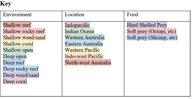
The results of the review indicate that tool use behaviours in Choerodon species are closely linked to ecological conditions where conventional foraging strategies prove inefficient or energetically demanding. Out of the 28 individual observations included in the analysis, 11 individuals (39%) exhibited clear tool use behaviours, such as employing coral rubble or flat stones to crack open the shells of hard-shelled prey like gastropods and bivalves. In contrast, 17 individuals (61%) relied exclusively on non-tool foraging strategies. Notably, tool use was significantly more frequent in reef systems characterised by low prey diversity and the dominance of well-defended prey types, where individuals appeared to benefit from enhanced foraging efficiency and reduced handling time.

A clear pattern emerged across reef environments: tool use behaviour was consistently observed in habitats where prey presented higher physical defences, supporting the idea that such behaviours are not random innovations but are context-dependent adaptations. The repeated occurrence of these behaviours across geographically distinct reef systems suggests an underlying evolutionary advantage. These findings align with the initial hypothesis that tool use in Choerodon species is an ecological adaptation that emerges in response to foraging challenges. Therefore, the results support the hypothesis, reinforcing the argument that these behaviours are adaptive strategies shaped by environmental pressures rather than isolated behavioural anomalies.

Tool use behaviour in non-human animals has long intrigued scientists for what it reveals about cognition, adaptability and the evolutionary emergence of complex behaviours. In marine ecosystems, such behaviour is both rare and under-documented compared to terrestrial environments, where primates and birds have historically dominated the discussion. This investigation focused on Choerodon wrasses, a genus within the Labridae family, and explored how ecological pressures might influence the emergence and persistence of tool use behaviour in reef fish. The core argument proposed is that tool use in Choerodon

species is an adaptive response to environmental complexity and prey-processing challenges, underpinned by cognitive flexibility and ecological opportunity.

Two key sources formed the foundation of this academic investigation. Jaishankar (Jaishankar, 2024) documented the use of anvils by Choerodon schoenleinii, commonly known as Blackspot Tuskfish, to break open mollusc shells, providing direct evidence of tool-assisted foraging in a wild reef fish. Their field-based observations linked this behaviour to prey availability and specific structural features of the habitat, such as the presence of flat, hard surfaces suitable for smashing. This demonstrated that such behaviours are not random but may be contingent on environmental affordances. Another crucial study by Brown and Laland (Brown & Laland, 2003) reviewed innovation and learning in fish, highlighting how complex environments select for behavioural plasticity. Their findings support the idea that coral reef habitats, with their intricate threedimensional structure and high prey diversity, create strong evolutionary pressures that favour innovation, such as tool use.

Other studies in the field further reinforce these ideas. For instance, Paśko (Paśko, 2010) reported memorybased tool use in six-bar wrasses, suggesting that reef fish may possess spatial memory capabilities that allow them to recall the location of suitable objects or locations for prey processing. Additionally, environmental enrichment, such as increased habitat complexity and access to varied stimuli, was shown to promote cognitive flexibility and exploratory behaviour in wrasses. These insights strengthen the claim that behavioural innovation in fish is not only ecologically driven but also shaped by cognitive adaptability. Similarly, Adam and Toledo (Adam & Toledo, 2025) proposed systematic experimental designs to study wrasses tool use under controlled conditions, aiming to determine whether such behaviours are innate, learned, or situational. Their proposal marks a significant step toward formalising research on marine cognition and behavioural evolution.

The data analysis in this investigation drew from peerreviewed journal articles, behavioural ecology reviews, and species-level databases such as FishBase and Fishes of Australia. Information was synthesised thematically, grouping factors such as environmental complexity, prey morphology, observed object manipulation, and cognitive indicators like problemsolving or innovation frequency. Due to the qualitative nature of available evidence, no statistical models

were applied. However, triangulation across academic literature, field observations, and ecological databases allowed for the cross-validation of behavioural patterns and increased the robustness of the analysis. While this method strengthens the credibility of inferred trends, a significant limitation remains: the analysis is constrained by the lack of experimental data, which restricts causal interpretations about the origins and functions of tool use in these fish.

Despite these promising findings, several limitations must be acknowledged. First, many primary studies on marine tool use remain behind paywalls, limiting full access to methodological data and raw data necessary for replication or critical appraisal. Second, much of the available evidence is anecdotal and lacks the rigour of experimental replication. For example, behaviours identified as “tool use” are not always described using consistent or universal definitions. Crain (Crain et al., 2013) argue for the adoption of a universal, cross-species definition of tool use to standardise research and improve comparability across taxa. Without such standardisation, it is difficult to evaluate whether observed behaviours qualify as true tool use or are simply opportunistic object interactions.

Additionally, while observational data provide valuable ecological insight, they cannot definitively determine cognitive mechanisms. The cognitive underpinnings of tool use in wrasses remain largely speculative. Current studies do not isolate variables such as learning, memory, or foresight in behavioural trials. Without controlled, repeated-measures experiments, it is difficult to confirm whether the behaviours demonstrate cognitive complexity, such as planning or problem-solving, or whether they are better interpreted as learned routines reinforced by environmental feedback. Jacobs and Osvath (Jacobs & Osvath, 2016) note that genuine tool use typically requires foresight, a level of cognitive processing not yet empirically demonstrated in reef fish.

The broader implications of these findings extend into conservation biology and marine ecology. As coral reefs face growing anthropogenic stress from overfishing, pollution, and climate change, behavioural adaptivity may become a key survival trait for reef-dwelling species. Tool use behaviour may serve as a proxy for cognitive resilience, indicating a species’ potential to adapt to changes in prey availability or habitat degradation. If Choerodon wrasses, and potentially other reef fish, can alter their foraging strategies in response to environmental changes, they may be more capable of surviving in rapidly shifting ecosystems.

Future research should focus on controlled experimental work to assess the cognitive scope of tool use in wrasses. Laboratory-based trials involving problem-solving tasks and manipulative challenges could isolate variables such as innovation, spatial memory, and learned behaviour. Furthermore, phylogenetic comparisons across Labridae species could help clarify whether tool use evolved independently or as a shared trait. Genomic and neurobiological analyses may also reveal underlying traits associated with innovation and adaptability. Long-term field studies would be valuable in determining whether tool use spreads through social learning, arises independently, or follows patterns of environmental consistency.

Conclusion

In conclusion, the emergence of tool use behaviour in Choerodon wrasses is an ecological adaptation as it represents an evolutionary response to environmental pressures shaped by habitat structure and prey availability. Although the current evidence is limited by accessibility issues and the observational nature of much of the data, this investigation provides strong preliminary support for the role of ecological adaptation in shaping behavioural complexity. Future interdisciplinary approaches combining ethology, ecology, cognitive science, and genetics will be essential to deepen our understanding of tool use and intelligence in marine organisms.

This study explored the relationship between ecological adaptation and tool use behaviour in Choerodon wrasses, aiming to understand if there is a relationship between ecological adaptation and tool use and how environmental complexity influences the evolution of innovative foraging strategies in marine species. Key resources consulted included primary databases, FishBase and Fishes of Australia, which provided consistent species-level ecological data, along with two pivotal peer-reviewed articles. TarielAdam (Adam & Toledo, 2025) offered field-based evidence of Choerodon schoenleinii using coral or rock anvils to process hard-shelled prey, illustrating direct tool use behaviour. Complementarily, Brown and Laland (2003) discussed how cognitive innovation in fishes is shaped by their ecological contexts, underscoring the evolutionary significance of behavioural flexibility in complex habitats.

The findings revealed that specific ecological pressures, such as prey availability, reef architecture, and dietary specialisation, likely create conditions favourable for the emergence of tool use in Choerodon

wrasses, which supports an environmental adaptation pathway. These behaviours appear in environments where mechanical manipulation of prey provides a clear foraging advantage, indicating a functional and adaptive basis. Therefore, it can be concluded that, notably, these behaviours were not isolated incidents but have consistently been reported across diverse reef systems, suggesting that tool use may be more widespread than previously assumed. Additionally, the reliance on habitats that provide structural elements like corals or rocks further highlights the role of environmental affordances in shaping behavioural responses.

Ultimately, this study reinforces a growing body of research on cognitive evolution in marine organisms, highlighting that intelligence and innovation are not exclusive to mammals or birds but can emerge in response to environmental challenges across diverse taxa. These insights expand our understanding of animal intelligence and underscore the importance of habitat preservation in maintaining the ecological conditions that support such behavioural richness.

Acknowledgements

Prof. Cullum Brown for his guidance, research and expertise in this area. Mr. Kathy Haigh for her assistance and encouragement. Dr Matthew Hill for his assistance and encouragement.

References

Adam, J. T., & Toledo, J. G. (2025). Tool use by New World Halichoeres wrasses

Brown, C. (2015). Fish intelligence, sentience and ethics. Animal Cognition, 18(1), 1–17. https://doi.org/10.1007/s10071-014-0761-0

Brown, C., & Laland, K. N. (2003). Social learning in fishes: A review. Fish and Fisheries, 4(3), 280–288. https://doi.org/10.1046/j.1467-2979.2003.00122.x

Crain, B. J., Giray, T., & Abramson, C. I. (2013). A Tool for Every Job: Assessing the Need for a Universal Definition of Tool Use. International Society for Comparative Psychology.

Floeter. (2018). Phylogenetic perspectives on reef fish functional traits. Wiley Online Library. https://onlinelibrary.wiley.com/doi/10.1111/brv.12336

Jacobs, I., & Osvath, M. (2016). Nonhuman Tool Use. Lund University, Lund, Sweden

Jaishankar, S. (2024, February 14). Anvil use by three wrasse species: Halichoeres hortulanus, Thalassoma jansenii, and Thalassoma lunare https://link.springer.com/article/10.1007/s00338-02402467-y

Paśko, Ł. (2010). Tool-like behavior in the sixbar wrasse, Thalassoma hardwicke (Bennett, 1830). Zoo Biology, 29(6), 767–773. https://doi.org/10.1002/zoo.20307

Biofiltration of agricultural runoff using Carrex Apressa

Brett Minkus Barker College

Waterways and other marine environments are severely impacted by agricultural runoff. This is due to its high concentration of phosphates and nitrates that allow for waterways to become dangerous to marine life. Specifically, piggery runoff is found to have high concentrations of these nutrients. This project investigated whether the native Australian plant Carrex Appressa could be used to filter out high concentrations of phosphates and nitrates from mimicked runoff samples. For this to be achieved, several concentrations of runoff were made relating to the average and put through the plant. The water was then later tested for phosphates and nitrates. The results showed that about ninety percent of phosphates and nitrates were removed from each solution run through the plant. This means that the Carrex Appressa is a highly effective biofilter and can be used to filter piggery runoff before entering waterways thus improving water quality of marine areas.

Literature Review

Agricultural run-off in general has lowered water quality in coastal areas due to the high amount of sediment and nutrients in this runoff (Australian Institute of Marine Science, 2000). Furthermore, when water is contaminated with runoff containing nutrients such as phosphates and nitrates it can promote blue green algal growth in waterways destroying marine life and potentially contaminating drinking water and making it dangerous for consumption (PDF, n.d.a)(DCCEEW, 2022). More specifically effluent from piggeries has high concentrations of nitrates and phosphates due to animal waste and excess feed, meaning when piggery effluent becomes runoff it can be harmful to waterways (Pub4-Effluent-IntensivePiggeries.Pdf, n.d.). An example of how these nutrients can harm our marine environments is the effect it has on the Great Barrier Reef, and how land practices are contributing to the disruption of the reef (Davis et al., 2016).

Specifically agricultural runoff from piggeries can be high in these nutrients, this is due to piggeries having high populations and animals receiving high energy feed in order to gain weight efficiently. Thus, runoff from piggeries can be detrimental to the health of waterways and to the water quality. The average amount of phosphorus in pig effluent is 850 mg/L and the average for nitrogen is 2175mg/L(PDF, n.d.-b)

Biofiltration is a filtration system where the filter medium consists of a plant that assists in extracting physical and chemical water pollutants that flow through the plant roots. The plant Carrex Apressa or ‘Tall Sedge’ was selected for the biofilter due to its

utilization in past experiments with filtrating stormwater, and more specifically, with its ability of removing phosphates and nitrates that are contained in stormwater(Herzog et al., 2021) Similarly, this plant is also used by Hornsby council in biofiltration of storm water and is highly recommended by professionals from Hornsby council (Naughton, 2025). Criteria used when selecting a plant for a biofilter in the project was that the plant must be able to survive in typical biofilter environment (sandy substrate and intermittent inundation) (AGSBS-A5Vegetation-Selection-for-Stormwater-Biofilters.Pdf)

Piggery effluent is difficult to attain as it is a biohazard in some situations and can give away key information about piggeries that may be sensitive, so attaining piggery runoff from a famer is quite difficult. Additionally effluent is difficult to track as it runs off farm into waterways, so collecting can be difficult and attaining an average can be tedious. However, creating solutions to mimic the concentrations and content of pig effluent can be achieved with greater ease. Using back marvel liquid fertiliser and potash phosphate and nitrate levels can be mimicked; Potash contains four percent phosphate and Black marvel contains 15.08% nitrates and 1.08% phosphates.

Scientific Research Question

To what extent can Carrex appressa (tall sedge) effectively remove phosphates and nitrates from agricultural runoff, specifically piggery run off, when used as a biofilter?

Scientific Hypothesis

When the contaminated water runs through the roots of the Carrex Apressa it will extract nitrates and phosphates from the water thus improving the water quality of the contaminated runoff.

Methodology

To simulate a range of nitrate and phosphate typically observed in piggery, five 2500mL synthetic runoff samples were prepared to represent a range lower and higher than the average (850mg/L phosphate and 2175mg/L nitrate concentration). Black marvel and potash were used as the nitrate and phosphate sources, whilst de- ionised water was used as the solvent. The concentration of each runoff sample was as follows: A(control)(P-0, N-0), B(P-425, N-1087.5), C(P-850, N-2175), D(P-1700, N-4350), and E(P-3400, N8700).

Making effluent concentrations and plant preparation

The average concentration of phosphorus and nitrogen was sourced from. The average concentration of nitrogen was 2175mg/L, and 850 mg/L for phosphorus. There was a control (A) which had no phosphorus or nitrogen concentration (de-ionised water), B - a lower concentration; P-425 mg/L, N1087.5mg/L (half the average), C - the average concentration; P-850mg/L, N-2175mg/L, D - a higher concentration; P-1700mg/L, N-4350mg/L(double the average), and E - a very high concentration; P3400mg/L, N-8700mg/L. To make these five sample groups two fertilisers were purchased as a source of nitrogen and phosphorus. These were Black Marvel Tomato and vegetable food liquid fertiliser and liquid Potash (fruit and bloom booster). The black marvel was 15.05% nitrogen and 1.08 percent phosphorus, and the Potash was 4% phosphorus. Using the formula appropriate amounts of the fertilisers was added to deionised water. Each solution was 2500mL.

15 Carrex Apressa plants of a similar size and same age were purchased. Each plant was removed, and plant roots were washed and soaked to remove all soil and nutrients from the roots. Plants were then placed back into their original plastic pots and filled with clear river sand. Each plant was watered with 100 mL of tap water per day up until the experiment was conducted. 15 plastic trays were placed under each pot to collect any drainage water.

Sample collection

Over a 14-day period the experiment was conducted. Fifteen plants were randomly divided into five groups of three, corresponding to the five different runs off treatments. On odd numbered days, each plant was

watered with 100mL of its respective run off solution at the top of the pot. After 45 minutes 20mL of drainage water was collected from the tray under the pot, stored, labelled and frozen for subsequent chemical analysis. On even numbered days the height of each plant was measured using a measuring tape. The height in millimetres of the tallest reed visible was measured from the soil surface to the tip. All data was recorded in a table.

Data collection

The methods used in attaining phosphate and nitrate data using the PASCO colorimeter consist of:

Nitrate test: Fill a 15 mL reaction tube with the sample and add one Zinc Foil Pack (A-6905). Cap and shake vigorously for exactly 3 minutes to ensure complete reduction of nitrate to nitrite (ezSample Snap VialNitrate (EZ-2333B), n.d.). Add 10 drops of A-6901 acidifier to a 25 mL sample cup to stabilize the solution. Carefully pour the treated sample into the cup, avoiding zinc or solid residue. Insert the ezSample Snap Vial tip into the bottom and snap it to fill, ensuring a small air bubble remains to aid mixing (PASCO Scientific, 2020). Mix by inverting several times. After waiting exactly 10 minutes for full colour development, insert the ampoule into a calibrated PASCO colorimeter and record the nitrate-nitrogen concentration.

Phosphate test: Fill the sample cup to the 25 mL mark with the water sample, then add 2 drops of A-8500 Activator Solution. This reagent reacts with to produce a measurable colour change (ezSample Snap Vial - Phosphate (EZ-2337), (PASCO Scientific, 2020). Cap and shake thoroughly to ensure full mixing. Insert the ezSample Snap Vial tip into the bottom and snap it against the side, filling the ampoule while trapping a small air bubble for mixing (PASCO Scientific, 2020). Invert the ampoule several times so the bubble moves end to end for even reaction. After wiping the vial clean, allow exactly 3 minutes for full colour development. Finally, place the ampoule into a calibrated colorimeter and read the phosphate concentration. Accurate calibration and timing are essential for reliable and reproducible data.

Due to time and available resources, chemical analysis was conducted on samples from days 1, 7 and 13. The triplicate samples for each concentration from each day were combined to make a 60mL composite sample for the P and N tests. Once each group of three was combined and labelled, then phosphate and nitrate levels were analysed using the Pasco colorimeter. Samples were initially tested and if phosphate and nitrate values fell outside the recommend values then

the samples were diluted with deionised water. The Colourimeter was calibrated prior to testing and the Pasco test method was followed. phosphate and nitrate levels were measured and results recorded in a table and a final concentration corrected for any dilution factor.

Data was analysed in terms of percentage of phosphates and nitrates removed during biofiltration as well as height gained by the plant over the 14-day experimental period.

Results

Table 1: Plant height increase measurements over 14 days, plants watered with different phosphate/nitrate solutions (Data with * removed from calculations as it was noticed that this plant appeared in poor health during the trial period)

Table 2: ANOVA comparing mean change in heights across the various treatment groups.

Nitrate Data

Table 3: Nitrate in and out measurements for different solutions

Phosphate data

Table 4: phosphates in and out measurements for different solutions

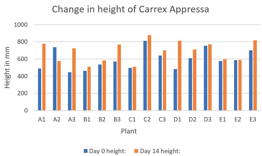
Figure 1: Carrex Appressa change in height: day 0 and day 14

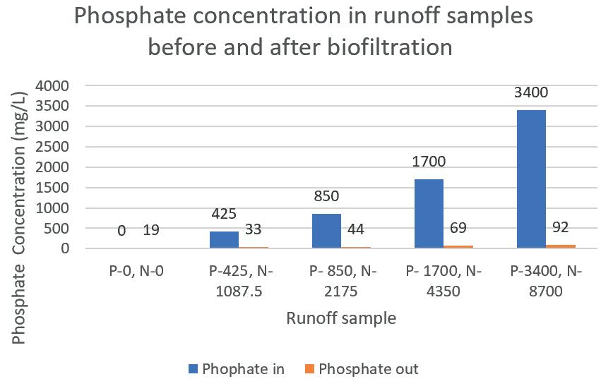
2: Phosphate concentration in and out of Carrex

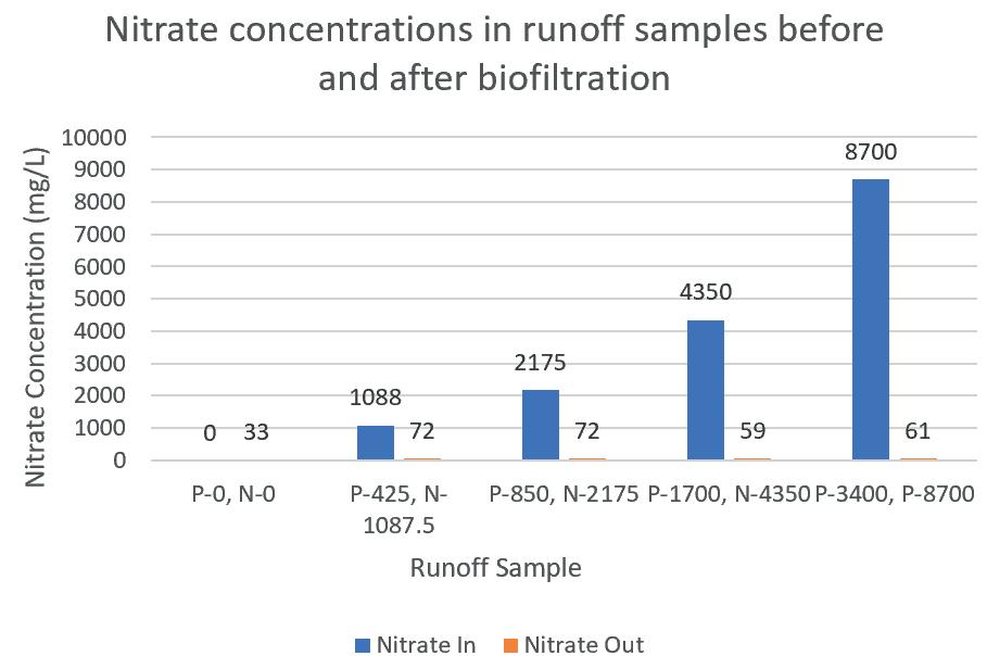
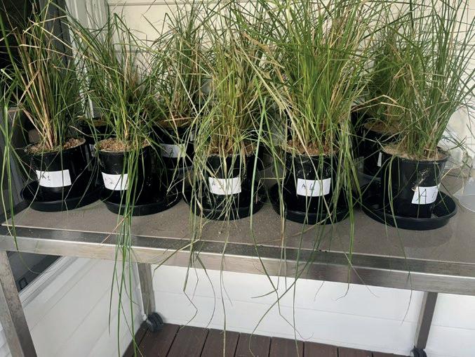
Discussion

The results from the experiment were very positive as the results reflected that around ninety percent of nitrates and phosphates were removed from each tested sample. It was discovered that even high amounts of phosphates and nitrates (Sample group EP: 3400 mg/L, N: 8700 mg/L) could be filtrated by Carrex Apressa plant and still not negatively impact the health of the plant. Therefor the hypothesis was confirmed meaning the Carrex Apressa effectively filtered out the phosphates and nitrates from the water as a biofilter. Due to time constraints, not all samples that were collected were tested. Samples tested were from the first day, seventh day and last day provided a reasonable estimate of how much effluent can be filtrated by the plant. However, as the results showed that the high concentration of runoff didn’t damage the plant, this still means that the limits of the plants filtration abilities has not been confirmed. Furthermore, as the plant still allows for less than ten percent of the nutrients to proceed through the plant, other filtration methods are still required to convert this water to drinking water. The excess nutrients still found in the water after filtration could have been due to the plant not being able to filtrate small concentrations of nitrates and phosphates, as plants do not work the same way as manufactured membrane

filtration systems. However, the control samples did detect small amounts of nitrate and phosphate concentrations in filtrated runoff samples, as seen in Table 3, Nitrate in and out measurements for different solutions and Table 4, phosphates in and out measurements for different solutions. This could have been because small amounts of nutrients or soil left in the plant roots contaminated the clean water, meaning roots should have been washed or cleaned using a more thorough method. Initially it was thought that the sand the plant was in added the additional nutrients to the clean water, but further tests were done to ensure this was not the case. The testing of the samples was slightly difficult as the equipment used was only accurate for the range provided and only detected very small amounts of phosphates and nitrates. The testing range for nitrates is o.25-2.00 mg/L(Palmer, n.d.-a) and for phosphates it was 0.20-8.00 mg/L(Palmer, n.d.-b). Each sample had to be diluted into water then tested. The results showed that percentage removal was slightly higher for the greater concentrations of phosphates and nitrates. For example, for phosphates group E (P-3400mg/L, N- 8700mg/L) ninety seven percent was removed by the plant however group B (P-450mg/L, N-1087.5mg/L) only had ninety two percent removed. This could be due to the plant being able to effectively filtrate in larger quantities meaning it is easier for nutrients to pass through the biofilter when watered down. A major limitation was that the piggery runoff samples were manufactured and only contained the nitrates and phosphates provided by liquid fertiliser rather than in its natural form.

The height of the plants was also measured on every second day, and it was found that there was no significant correlation between plant health and nutrient concentration. This was discovered through a statistical test as the P- value was below 0.05 (Table 55), this means there was no specific correlation between the data points this means there was a significant difference between change in height. However, recording the height did allow for observations to be made about the over -all health of each plant. Furthermore most plants did grow in height over the time period (Figure 1- Carrex change in height: day 0 and day 15) which means plants did have access to nutrients in order to grow taller. No group of plants were negatively impacted because of the testing however some individual plants did not respond well being transplanted from soil to sand. For example, plant A2 recorded negative height gain and did not appear as large as the other plants at the start of the experiment. This could have been because it was not as mature as the other plants. If this experiment were to be repeated all plants would have to have been germinated and of the same age,

unfortunately due to the resources that were available, 15 young Carrex Apressa of similar ages or maturity were purchase. This was effective for most of the other plants but A2, C3 and E2 (Table 1- Plant height increase measurements over 14 days, plants watered with different phosphate/nitrate solutions)were the only ones that recorded negative height gain and were plants that were observed as less healthy as others (Table 1- Plant height increase measurements over 14 days, plants watered with different phosphate/nitrate solutions). Furthermore, plant height did not increase according to the amount of phosphate and nitrates administered to the plant, however through observation the plants with higher phosphate and nitrate levels looked greener and healthier.

Conclusion

The key findings of this research project are thatCarrex Apressa removed approximately ninety percent of nitrates in runoff samples that varied in concertation from 0 to 8700 Mg/L. Carrex removed approximately ninety percent of phosphates in runoff samples that varied in concertation from 0 to 3400 mg/L. Carrex Apressa was trialed to examine if it could be used as a biofilter to remove nitrates and phosphates from mimicked piggery runoff. Through the collection and analysis of many samples the plant removed around ninety percent of the contaminants from the runoff. It was found that this did not correspond with the growth in height of the plant, yet plants with greater concentration of phosphates and nitrates were observed as greener and healthier. However, there were some limitations to this experiment. The plants purchased for the experiment were not all of the same size and maturity due to a limited supply, however this only notably effected the height data of some plants. Similarly smaller less developed plants were disadvantaged as they struggled from the change of environment from soil to sand which further affected the height data for these plants. Furthermore, not all of the samples that were collected were tested due to time pressures and lack of equipment. If all samples had been able to be tested, this could have enabled a more detailed data set that could have provided more detailed information. However, with the samples and data that was collected, it was found that Carrex Apressa effectively removes contaminants such as phosphate and nitrates

which are present in piggery runoff in high concentrations, Thus, being found to be an environmentally friendly method to filter this runoff using a readily available plant filter.

Acknowledgements

I would like to sincerely thank Mrs Kathy Haigh for her immense support and assistance throughout my research project. Thank you to her for all her feedback and insight into how to improve the project.

References

AGSBS-A5-Vegetation-selection-for-stormwaterbiofilters.pdf. (n.d.). Retrieved June 24, 2025, from https://watersensitivecities.org.au/wpcontent/uploads/2016/06/AGSBS-A5-Vegetation-selectionfor-stormwater-biofilters.pdf

Davis, A. M., Pearson, R. G., Brodie, J. E., & Butler, B. (2016). Review and conceptual models of agricultural impacts and water quality in waterways of the Great Barrier Reef catchment area. Marine and Freshwater Research, 68(1), 1–19. https://doi.org/10.1071/MF15301

ezSample Snap Vial Nitrate (EZ-2333B). (n.d.).

ezSample Snap Vial Phosphate (EZ-2337). (n.d.).

Herzog, T., Mehring, A., Hatt, B., Ambrose, R., Levin, L., & Winfrey, B. (2021). Pruning stormwater biofilter vegetation influences water quality improvement differently in Carex appressa and Ficinia nodosa. Urban Forestry & Urban Greening, 59, 127004. https://doi.org/10.1016/j.ufug.2021.127004

Palmer, R. (n.d.-a). ezSample Snap Vial Nitrate • EZ2333B. PASCO Scientific. Retrieved June 24, 2025, from https://www.pasco.com/products/sensors/environmental/ez sample-snap-vial-nitrate

Palmer, R. (n.d.-b). ezSample Snap Vial Phosphate • EZ2337. PASCO Scientific. Retrieved June 24, 2025, from https://www.pasco.com/products/sensors/environmental/ez sample-snap-vial-phosphate

PDF. (n.d.-b). Retrieved June 24, 2025, from https://australianpork.com.au/sites/default/files/202302/Piggery-Manure-and-Effluent-Management-andResure-Guidelines.pdf

Pub4-effluent-intensive-piggeries.pdf. (n.d.). Retrieved November 29, 2024, from https://www.waterquality.gov.au/sites/default/files/docume nts/pub4-effluent-intensive-piggeries.pdf

How do different postharvest treatments (sugar, bleach, water regulation) effect the vase life and colour stability of white carnations, measured by CIELAB colorimetry?

Melissa Li Barker College

This study investigated aims to compare the postharvest treatment used in maintain the flower colour stability of cut flowers by testing different vase solutions (30ml) and storage conditions. The key question was whether sugar, bleach, water regulation, or high humidity and low temperature could best prolong the colourings change. Freshly cut flowers were randomly divided into groups: one placed in water regulation (control), others in solutions containing sugar (nutrient source), bleach (antimicrobial). Another group was stored in a fridge to assess temperature effects of low temperature and high humidity. Cut flower quality was monitored every 2 days for wilting, petal discoloration, and water uptake. Results showed that flowers in 3%sugar solution had the most stable colour spectrum (up to % more than the control), as sugar provided nutrients while bleach reduced bacterial growth. Refrigeration further extended freshness by slowing metabolic activity. In contrast, flowers in water regulation wilted fastest. The study concludes that a 3% sugar solution, was best at maintaining cut flower colour stability by improving nutrient availability, inhibiting microbes, and reducing decay. (how the sugar improved the colour stability in a scientific point of view)

Literature Review

Cut flower industry is quickly rising as it was valued at more than 34 billion USD in 2019 according to data. The five main types of cut flowers are rose, carnation, lilium, chrysanthemum, and gerbera (Markets, 2021). Cut flowers are a significant part of floral industries, yet their vase life is limited due to physiological and environmental factors. Understanding the mechanisms that influence bloom time, colour stability, and postharvest treatments is essential for improving flower longevity (Vehniwal & Abbey, 2019). This experiment examines key factors affecting cut flower senescence, the science behind colour changes, common preservation methods, and the role of colorimetry in quantifying these changes. The focus will be on white carnations (Dianthus caryophyllus), a flower due to their year-round availability and sensitivity to treatments (Jędrzejuk et al., 2013).

Factors Affecting Bloom Time and Longevity

The lifespan of cut flowers is influenced by genetic, environmental, and biochemical factors. Flowering time is regulated by photoperiodism, where light quality and duration trigger floral transition (Kim et al., 2008). The genes CONSTANS (CO) and FLOWERING LOCUS T (FT) play crucial roles in this process (Putterill et al., 2004). Once cut, flowers undergo accelerated senescence due to water stress, microbial growth, and ethylene exposure (Chen et al., 2024). Sugar level is another critical factor; exogenous

sucrose application delays senescence by maintaining cellular respiration (Ohto et al., 2001). However, excessive sugar can promote microbial growth, necessitating antimicrobial agents like sodium hypochlorite (NaOCl) and hydrogen peroxide (H₂O₂) (Meral et al., 2024). Yoo et al. (2016) demonstrated that a combination of NaOCl and benzyl adenine (a cytokinin) extended chrysanthemum vase life by reducing bacterial blockage in xylem vessels.

Why is Bloom Length Important?

Extending the vase life of cut flowers has economic and aesthetic benefits. The global floral industry relies on long-lasting blooms to reduce waste and improve customer satisfaction (Abbie, 2024). Additionally, flowers positively impact human emotions, with studies showing that their presence enhances mood and reduces stress (Haviland-Jones et al., 2005). Thus, improving postharvest longevity has both commercial and psychological value.

Colour Changes in Cut Flowers

Once cut, flowers undergo visible colour shifts due to pigment degradation, pH changes, and oxidative stress. White carnations, for instance, may develop pink or yellow hues as chlorophyll breaks down and anthocyanin production increases (Jędrzejuk et al., 2013). This phenomenon is accelerated by ethylene, a plant hormone that promotes senescence (Jones, 2001).

Measuring Colour Changes Using CIELAB (L, a, b) Values

Colorimeters quantify flower colour changes using the CIELAB system, which defines colour in three dimensions:

- L (Lightness): Ranges from 0 (black) to 100 (white).

- a (Red-Green) Positive values indicate red; negative values indicate green.

- b (Blue-Yellow): Positive values indicate yellow; negative values indicate blue (X-Rite, n.d.).

Tracking these values over time helps assess the senescence-related colour shifts. For example, a decrease in L indicates darkening, while an increase in b suggests browning.

Common Postharvest Treatments

Several methods are used to prolong cut flower freshness in the researches: Antimicrobial Agents(bleach), Sodium hypochlorite (NaOCl) and hydrogen peroxide (H₂O₂) reduce bacterial growth in vase water (Meral et al., 2024), Sugar Solutions which provide energy to flowers but require antimicrobials to prevent microbial proliferation (Ohto et al., 2001), Low temperature, high humidity which delay senescence by suppressing ethylene effects (Yoo et al., 2016). Water Circulation Systems by prevent vascular blockage, improving water uptake (Chen et al., 2024).

Conclusions

Understanding the factors influencing cut flower longevity from genetic regulation to postharvest treatments is crucial for improving floral industry practices. White carnations serve as an ideal model due to their sensitivity to senescence and accessibility. Future research should integrate colorimetric analysis to better quantify treatment efficacy, providing a more objective measure of flower quality over time.

Scientific Research Question

How do different postharvest treatments (sugar, bleach, water regulation) effect the vase life and colour stability of white carnations, measured by CIELAB colorimetry?

Scientific Hypothesis

3% carbohydrate status will be the most effective treatment in maintaining flower colour stability,

carbohydrate status, Bleach concentration and water regulation. As it directly influences nutrient uptake and metabolic processes, which are essential for flower longevity and extending its flowering time. Articles on carbohydrate status are also commonly seen to suggest that 3% carbohydrate status extend the flowering time of cut flowers the best.

Methodology

The experiment is conducted in a controlled environment using cut flowers of the same species and initial quality to ensure consistency. The carnations will be divided into groups of 3 stems, with each group subjected to a different method aimed at compared which method will extend the flowering time the best. For water relation acting as the control, the water will be changed once every 2 days to maintain optimal hydration and prevent microbial growth, as supported by Chen et al. (2024). For carbohydrate status, sugar treatments of the concentration of 3% are used to provide energy and delay senescence. To evaluate the effects of temperature and humidity, one group of flowers will be stored in a refrigerator to slow metabolic processes and reduce water loss. For pathogen management, bleach of 50ppm is added to the water to inhibit microbial growth and maintain water quality. The independent variable will be the different methods applied to extend flowering time, while the dependent variable will be the duration of flowering time, measured with the b value and water uptake. Controlled variables, including light exposure, initial flower quality, and humidity and the amount of water will be kept constant across all groups to ensure accurate comparisons. Data will be collected every 2 days by monitoring and recording flowering time and assessing flower quality using visual indicators such as colour change to the naked eye and colorimeter. The leaves on all stems are removed and the end is cut in a 45-degree angle then placed in a test tube with 30ml of the independent variable. The amount of water uptake will be measured every 2 days, and the solution should be changed after every measurement while taking a petal from the colour and measuring it’s L, a, b value with a colorimeter and recording it in a table. Repeat this procedure until day 6 (with the first day of setting up the experiment being day 0).

Results

Table 1: "Split sample" in bleach treatment indicates measurement uncertainty.

Table 2: (Stable L value (94–96) across all treatments. 3% carbohydrate showed slight increase (95.0 → 95.7), suggesting maintained colour

Table 3: This table indicates how browning is relevant to water uptake and the b-value

Table 4: Summary data change over a 6 day period.

Table 5: Further showcase the relevance between b-value and browning hence the dependent variable

Discussion

Sugar Treatment Efficacy

The superior performance of the 3% sugar treatment aligns with established physiological principles. Sucrose acts as an energy source, maintaining cellular respiration and delaying senescence (Ohto et al., 2001). The results showed a reduction in browning (b = −1.44), likely due to suppressed chlorophyll degradation and oxidative stress (Jędrzejuk et al., 2013). Additionally, the highest water uptake (5.2 mL) suggests that carbohydrates may improve hydraulic conductivity, mitigating xylem blockage which is a common issue in cut flowers (Vehniwal & Abbey, 2019). These findings corroborate studies on chrysanthemums, where sugar combined with low temperature high humidity to maintain the stability of colour (Yoo et al., 2016).

Low Temperature Trade-offs

While low temperature storage inhibited browning, its low water uptake (2.3 mL) indicates restricted transpiration and potential cold stress. This aligns with Chen et al. (2024), who noted that high humidity alone cannot compensate for reduced metabolic activity at cooler temperatures. The absence of browning suggests ethylene suppression (Jones, 2001), but the trade-off in hydration limits its standalone use.

Bleach Treatment Variability

The inconsistent results of the 50-ppm bleach treatment (e.g. split sample on Day 8) may reflect microbial adaptation or uneven distribution. Sodium hypochlorite’s antimicrobial effects are well documented (Meral et al., 2024), but its efficacy depends on concentration and exposure time. The data suggest that higher or more frequent doses may be needed to sustain sterility without damaging tissues.

Water Regulation Limitations

The increased browning (b= +1.19) in water regulated flowers likely stems from oxidative stress and microbial proliferation. Without antimicrobials or nutrients, vascular occlusion accelerates, as noted in roses (Proietti et al., 2022). This underscores the importance of additive treatment in cut flower care.

Comparison with Prior Research

The results support and expand upon key studies, with energy supply which refers to the success of carbohydrates mirrors Ohto et al. (2001), who linked exogenous sugars to delayed floral senescence in Arabidopsis.

Ethylene Management: The anti-browning effect of low temperature parallels Jones (2001), who highlighted ethylene’s role in petal aging.

Microbial Control: The bleach variability echoes Meral et al. (2024), emphasizing concentration dependent efficacy.

Notably, the research focus on colorimetric changes (via CIELAB) adds a novel dimension, as most studies prioritize vase life over quantitative colour metrics (XRite, n.d.).

Limitations and Uncertainty

Sample Size: Small replicates (n=3 per treatment) may affect statistical power.

Subjectivity: Browning scores relied on visual assessment; future work could use spectrophotometric standards.

Environmental Controls: Unmeasured variables (e.g., ambient ethylene) may have influenced results.

Future Research Directions

Building on this study, future work should investigate hybrid preservation solutions (e.g. 3% sugar with lowdose bleach) to simultaneously address hydration and microbial growth. The interaction between carbohydrate metabolism and pigment degradation particularly the mechanism behind reduced browning (b -value), warrants biochemical analysis using HPLC. Additionally, pulsed different temperature protocols could optimize the trade-off between ethylene suppression and water uptake observed in low-temperature storage. Expanding this research to commercially popular flowers like roses or lilies, while incorporating consumer preference surveys, would enhance practical application of this research. These steps would advance both the scientific understanding and real-world implementation of cut flower preservation.

Practical Implications

For florists and consumers, these findings are suggested Adopt carbohydrate solutions (3% sugar) for routine use, Reserve bleach for short-term displays due to inconsistency and avoid water-only storage to prevent rapid deterioration.

Therefore, this study demonstrates that carbohydrate supplementation effectively prolongs cut carnation freshness by addressing hydration, energy, and oxidative challenges. While low-temperature and bleach treatments offer niche benefits, their limitations highlight the need for tailored solutions. Future research should refine formulations and integrate advanced monitoring tools (e.g. CIELAB, microbial assays) to optimize postharvest care.

Conclusion

This study evaluated the effects of four postharvest treatments: 3% carbohydrate solution, 50 ppm bleach, low temperature and high humidity storage, and water regulation, on the longevity and quality of cut white carnations. The results demonstrated differences in efficacy, with the 3% carbohydrate treatment emerging as the most effective method for prolonging vase life. This treatment showed the highest water uptake (total of 45ml), reduced Browning (b = -1.44), and supported stem elongation (+3.5 cm), suggesting optimal hydration and delayed senescence.

In contrast, low temperature storage effectively prevented browning but significantly limited water uptake (2.3 ml), indicating potential trade-offs between hydration and microbial control. The bleach treatment exhibited inconsistent results, likely due to microbial resistance or sample variability, while water regulation alone led to increased browning (b = +1.19) and moderate dehydration. These findings align with prior research on carbohydrate-based preservatives (Ohto et al., 2001) and highlight the importance of balanced antimicrobial and nutrient supplementation in cut flower care.

Ultimately, the result supports the use of carbohydrate solutions for maintaining cut flower freshness, though further research could optimize concentrations and assess long term microbial effects. The data provide practical insights for florists and consumers seeking to extend floral displays.

Acknowledgements

I would also like to acknowledge the Science Extension teachers, in particular Mrs Kathy Haigh for her mentoring throughout my research and experiment which has expertly guided me through the project and Dr Matthew Hill for the extensive knowledge on the data and analysis. I would also like to extend my acknowledgment to the Science department for the provision and use of equipment.

References

5 Easy Ways to Lengthen the Life of your Cut Flowers The Plant Gallery. (n.d.). Retrieved February 24, 2025, from https://theplantgallery.com/5-easy-ways-to-lengthen-thelife-of-your-cut-flowers/

Abbie. (2024, May 17). How to Recycle and Dispose of Flowers | Waste Managed. Waste Management Services | Recycling | Waste Managed. https://www.wastemanaged.co.uk/our-news/funeral/howto-recycle-and-dispose-of-flowers/

Chen, C.-N., Ko, Y.-C., & Hsu, F.-C. (2024). Enhancing Aesthetics and Prolonging Lifespan of Cut Flowers with an Innovative Water Circulation Filtration System. Sensors and Materials, 36(5), 1747. https://doi.org/10.18494/SAM4790

Flowering Plant Life Cycle | Life Cycle of a Plant. (n.d.). Twinkl. Retrieved November 4, 2024, from https://www.twinkl.com.au/teaching-wiki/flowering-plantlife-cycle

Haviland-Jones, J., Rosario, H. H., Wilson, P., & McGuire, T. R. (2005). An Environmental Approach to Positive Emotion: Flowers. Evolutionary Psychology, 3(1), 147470490500300109. https://doi.org/10.1177/147470490500300109

Jędrzejuk, A., Rochala, J., Dolega, M., & Łukaszewska, A. (2013). Comparison of petal senescence in forced and unforced common lilac flowers during their postharvest life. Acta Physiologiae Plantarum, 35(6), 1785–1796. https://doi.org/10.1007/s11738-013-1216-y

Jones, R. (2001). Caring for Cut Flowers. Landlinks Press.

Kim, S. Y., Yu, X., & Michaels, S. D. (2008). Regulation of CONSTANS and FLOWERING LOCUS T Expression in Response to Changing Light Quality. Plant Physiology, 148(1), 269. https://doi.org/10.1104/pp.108.122606

LAB Color Space and Values | X-Rite Color Blog. (n.d.). XRite. Retrieved June 10, 2025, from https://www.xrite.com/blog/lab-color-space

Meral, E. D., Arman, Ç., Süslüoğlu, Z., & Arslan, S. (2024). The Effect of Sodıum Hypochlorite and Hydrogen Peroxide on the Vase life of Cut Rose Flowers. Türk Doğa ve Fen Dergisi, 13(4), Article 4. https://doi.org/10.46810/tdfd.1563639.

Ohto, M., Onai, K., Furukawa, Y., Aoki, E., Araki, T., & Nakamura, K. (2001). Effects of Sugar on Vegetative Development and Floral Transition in Arabidopsis. Plant Physiology, 127(1), 252–261.

Proietti, S., Scariot, V., De Pascale, S., & Paradiso, R. (2022). Flowering Mechanisms and Environmental Stimuli for Flower Transition: Bases for Production Scheduling in Greenhouse Floriculture. Plants, 11(3), Article 3. https://doi.org/10.3390/plants11030432

Putterill, J., Laurie, R., & Macknight, R. (2004). It’s time to flower: The genetic control of flowering time. BioEssays, 26(4), 363–373. https://doi.org/10.1002/bies.20021

Vehniwal, S. S., & Abbey, Lord. (2019). Cut flower vase life – influential factors, metabolism and organic formulation. Horticulture International Journal, 3(6). https://doi.org/10.15406/hij.2019.03.00142

Yoo, Y. K., Oh, H. J., Roh, Y. S., & Kim, I. K. (2016). Effects of Pretreatment of NaOCl, Sucrose, and Benzyladenine on Vase Life and Quality of Cut Flower in Standard Chrysanthemum ‘Jinba.’ Journal of Korean Society for People, Plants and Environment, 19(6), 559–566. https://doi.org/10.11628/ksppe.2016.19.6.559